Week 3 - Solving second order ODEs

Objective: To simulate the transient behavior of a simple pendulum by solving a second-order ODE

Theory:
A simple pendulum consists of a relatively massive object hung by a string from a fixed support. It typically hangs vertically in its equilibrium position. The massive object is affectionately referred to as the pendulum bob. When the bob is displaced from equilibrium and then released, it begins its back and forth vibration about its fixed equilibrium position. The motion is regular and repeating, an example of periodic motion.

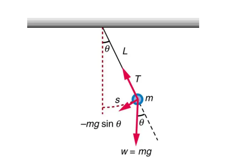
The equation of a simple pendulum is given by:
`(d^2theta)/(dt^2) + (b/m)(d theta)/dt +(g/l) sin(theta) = 0`

In the above equations,
g = gravity

b = damper coefficient

L = length of the pendulum

m = mass of the ball

To solve this second order ODE, following process is performed:

`(d^2theta)/(dt^2) + (b/m)(d theta)/dt +(g/l) sin(theta) = 0`

Let us assume:

`theta = theta_1`

So, `(d theta)/dt = (d theta_1)/(dt) = theta_2`

Differentiating both sides,

Put these expressions in the above second order ODE, we get:

`(d theta_2)/(dt) + (b/m) (theta_1) + (g/l) sintheta_1`

Based on this, we can now form a matrix system for getting the solution vector:
`(d theta)/dt = [[d theta_1], [d theta_2]] = [[theta_2],[(-b/m)theta_2 - (g/l)sin theta_1]]`..........Eq 1

A python script is then used to find the values of angular dispplacement and angular velocities.

Code explaination:

1) Numy, scipy, math and matplotlib.pyplot are imported.

2) The input parameters are defined with b = 0.05, g = 9.81 m/s^2, l = 1m, m = 1m.

3) A function by the name 'pend' is defined such that it returns equation 1.

4) Finally, odeint from scipy is used to solve the ODE.

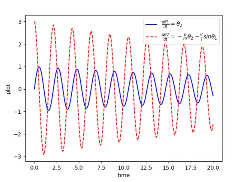
5) The solution vector are plotted as a function of time.

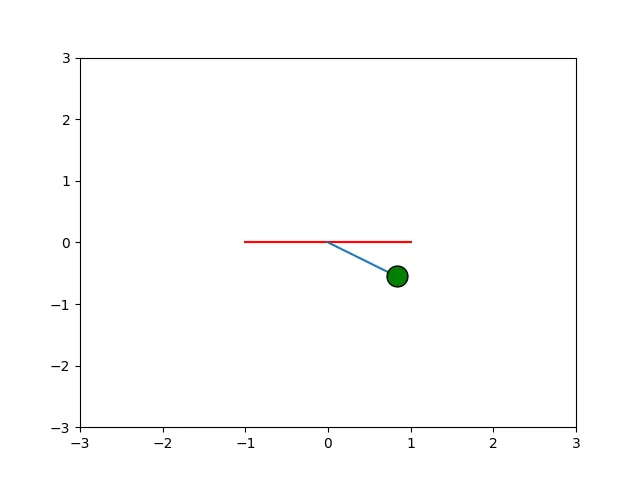
6) The angular velocity and displacement entries are seperated and the point of interest is found using simple trignometry as follows: X1 = L*`sin(theta_1)`, Y1 = `L*cos(theta_1)`

7) A plot of the pendulum is generated using the markers in python and each figure is saved into a seperate .png file and the files are stitched to create an animation.

import math
import numpy as np
from scipy.integrate import odeint
import matplotlib.pyplot as plt

#define the problem as ode
def pend(theta,t,b,g,l,m):
	dtheta_1 = theta[1]
	dtheta_2 = -(b/m)*theta[1]-(g/l)*math.sin(theta[0])
	dtheta = [dtheta_1,dtheta_2]
	return(dtheta)

#defining input parameters: g (m/s^2), l = 1m, m = 1 kg
b = 0.05
g = 9.81
l = 1
m = 1

#defining time array, t = 20s
t = np.linspace(0,20,300)

#defining initial conditions:
theta_0 = [0,3]

#solving ODE using the given graph
theta = odeint(pend,theta_0,t,args = (b,g,l,m))

print(theta)

#plot of displacement and angular velocity

plt.plot(t,theta[:,0],'b-',label=r'$\frac{d\theta1}{dt}=\theta_2$')
plt.plot(t,theta[:,1],'r--',label=r'$\frac{d\theta2}{dt}=-\frac{b}{m}\theta_2-\frac{g}{l}sin\theta_1$')
plt.xlabel('time')
plt.ylabel('plot')
plt.legend(loc='best')
plt.show()

#to plot the pendulum, we can use the following loop
angular_disp = []
angular_velocity = []
ct = 1

for i in range(0,len(t)):

	temp = theta[i,0]
	temp_2=theta[i,1]
	angular_disp.append(temp)
	angular_velocity.append(temp_2)

for j in range(0,len(t)):
	x0 = 0
	y0 = 0
	x1 = l*math.sin(angular_disp[j])
	y1 = -l*math.cos(angular_disp[j])


	plt.figure()
	plt.plot([-1,1],[0,0],color = 'r')
	plt.plot([x0,x1],[y0,y1])
	plt.plot(x1,y1,marker = "o",markerfacecolor = 'g',markeredgecolor = 'k',markersize = 15 )
	plt.xlim([-3,3])
	plt.ylim([-3,3])
	ct = ct+1
	filename = str(ct) + '.png'
	plt.savefig(filename)
	

Results:

Conclusion: The given second order ODE has been solved.