Elasto-Plastic Material modeling from raw data in LS-DYNA

Objective:

Modeling of elasto-plastic material and validation of the same using LS-DYNA

Introduction:

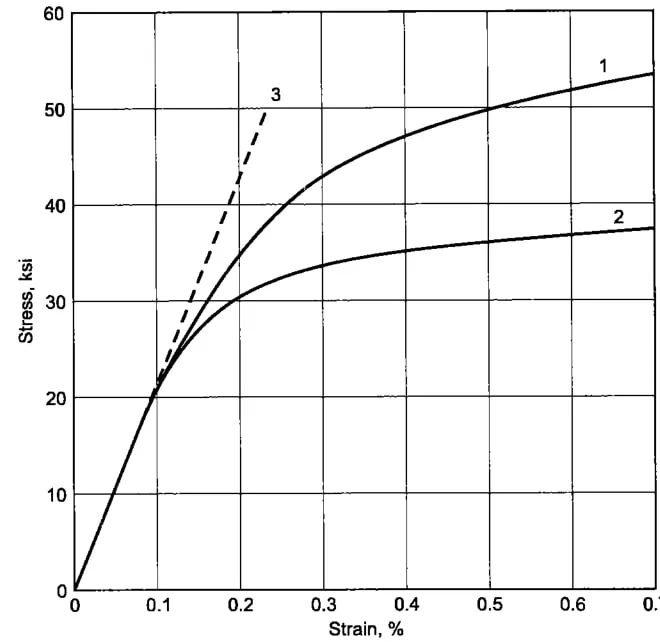
The stress-strain curve has been provided to us with true stress-true strain values for graphite iron casting. The initial step is to choose the curve and extract the data using a data digitizer. For this case, curve 2 was chosen to be extracted using a data digitizer.

MAT_024 material model and MAT_018:

MAT_018 is used to define the plasticity model using power law for plasticity which says that:

`sigma_y = kepsilon^n`

Here, `k`= Strength coefficient

`n`= Hardening coefficient

`epsilon`= Total strain

Using the above-mentioned equation, we get the behavior of our stress-strain curve for metals.

Likewise, MAT_024 is also used to describe material plasticity for a model. This form of bi-linear/multi-linear form of the stress-strain curve needs either tangent modulus value or a curve in the input card. Care should be taken while defining a curve. Using an optimum number of points to define the curve, fitting the curve using mathematical tools to avoid noisy data are the steps to be taken if a curve is defined for this card. Hence, defining a multi-linear/bi-linear curve using smoothed out data successfully captures the accuracy of material behavior with this card.

PROCEDURE:

The data is given to us in an image form and to extract values out of the same, data_digitizer is used. The given values are true stress- true strain values are in units ksi and % respectively. This form of data is converted to N/M^2 and strain value. Further, the units for the given problem statement are described in kg-mm-ms and the stress values are converted accordingly. The young's modulus given for this material is 20.9E+06 psi (144 GPa). Since the curve should have the only plasticity described, the yield point is taken as the starting point for the simulation. The true strain values are converted to effective strain values using the formula:

Effective plastic Strain = Total true strain - true stress/E

We use these values as the input for our analysis.

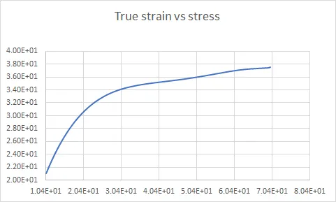
Fig: True stress vs true strain plot in the model.

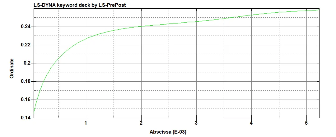
Fig: Effective strain vs Effective stress

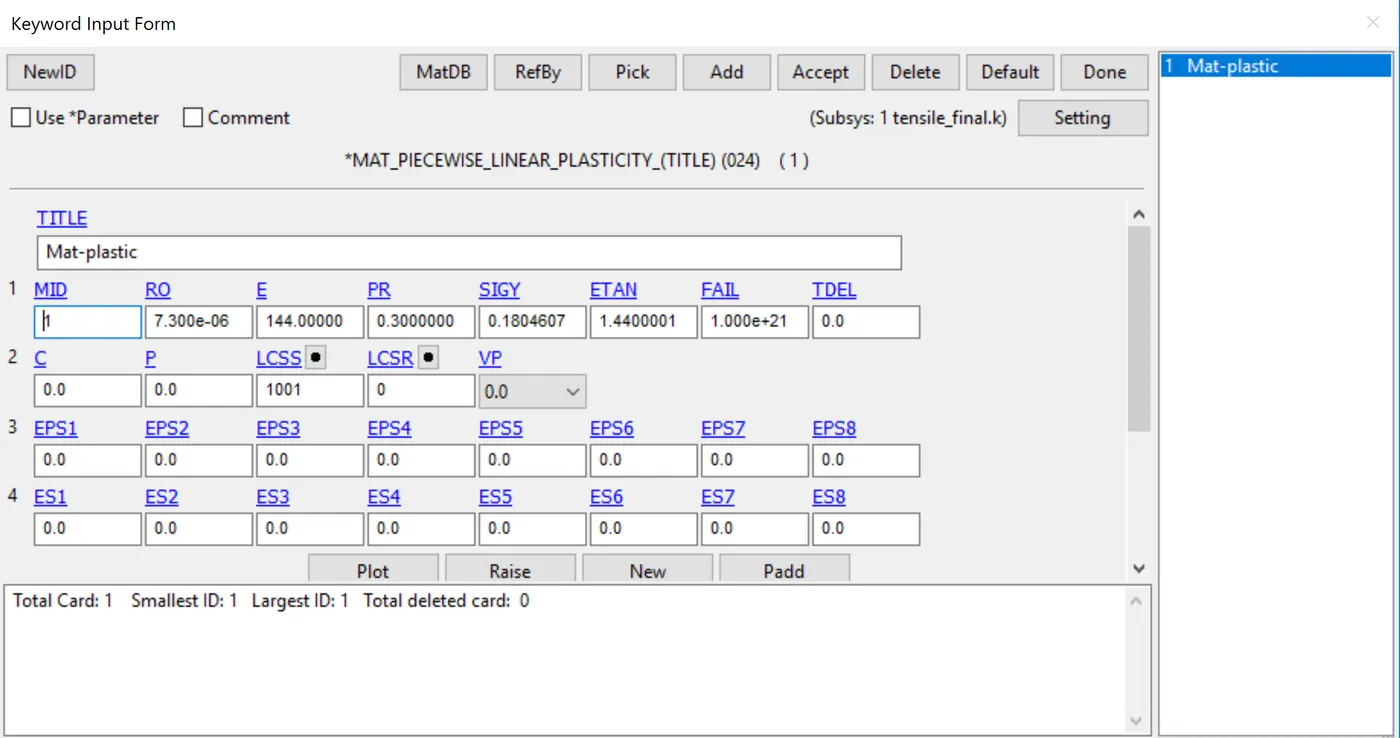
Yield stress is used as per the graph value and the tangent modulus is 1% of the elastic modulus. Since a curve has been given for LCSS, these values would mostly be ignored for our simulation. All the values are converted in kg-mm-ms unit system and the stress-strain data is converted to the given units. The data has been edited to take the hardening portion of the curve after eliminating the elastic points. LS-DYNA takes this curve and using the elastic modulus and the PR, computes the elasto-plastic curve for simulation. The PR taken for this material is 0.3 and the Elastic modulus values are 144 GPa accordingly.

Now, these values are input to LS Dyna in the MAT_024 card.

Shell section properties are used for the tensile test sample with 1.5 mm thickness. The total displacement is given in the form of a curve to the sample by first defining a node set and then inputting the required curve using the BOUNDARY_PRESCRIBED_NOTION card.

Two BOUNDARY_SPC cards have been used for constraining the left side of the sample and center nodes of both ends.

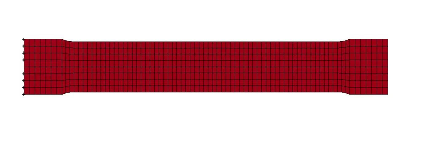
Fig: Left end constraints

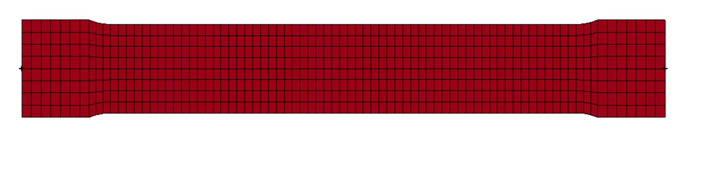
Fig: Two center constraints

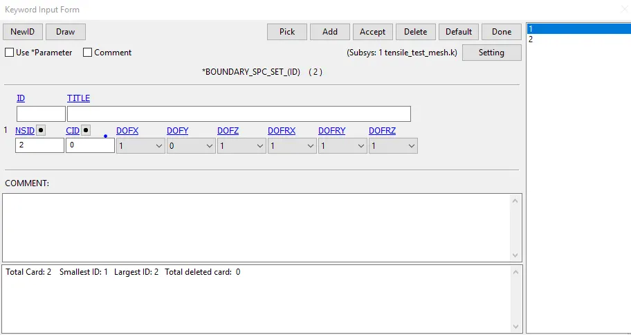
Fig: Boundary SPC card.

The two end constraints have been given no degree of freedom whereas the left constraints have been given DOF in the Y direction because the sample gets compressed in the Y direction from both sides during the test.

Generally, the tensile test is a slow process and can be considered as a quasi-static process. Hence, implicit analysis is used for this test. Using the *CONTROL_IMPLICIT_AUTO card, the number of iteraiton have been set to 100. The initial step size is 0.001.

RESULTS AND DISCUSSION:

EFFECTIVE STRESS:

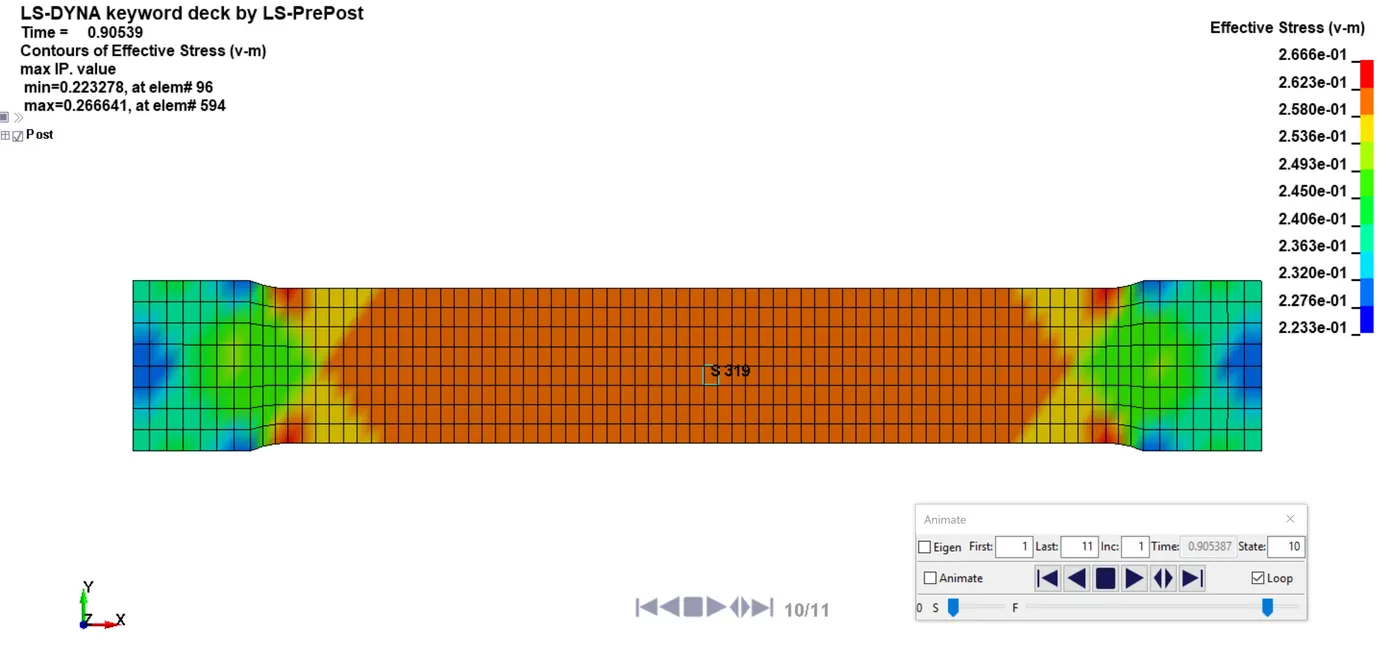
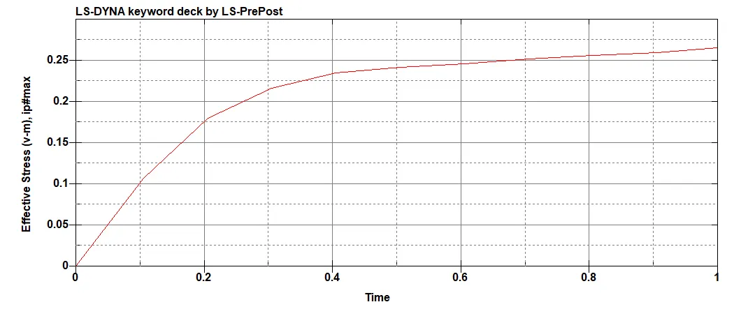
The figures below show the specimen in tension. The last time step is chosen for contour display and the element in the middle of the specimen is chosen for showing the effective stress curve. Given the amount of strain for this problem, necking is not expected from this specimen. However, as can be seen from the graph, the stress value observed is more than the yield stress and hence, plastic deformation is expected.

EFFECTIVE STRAIN:

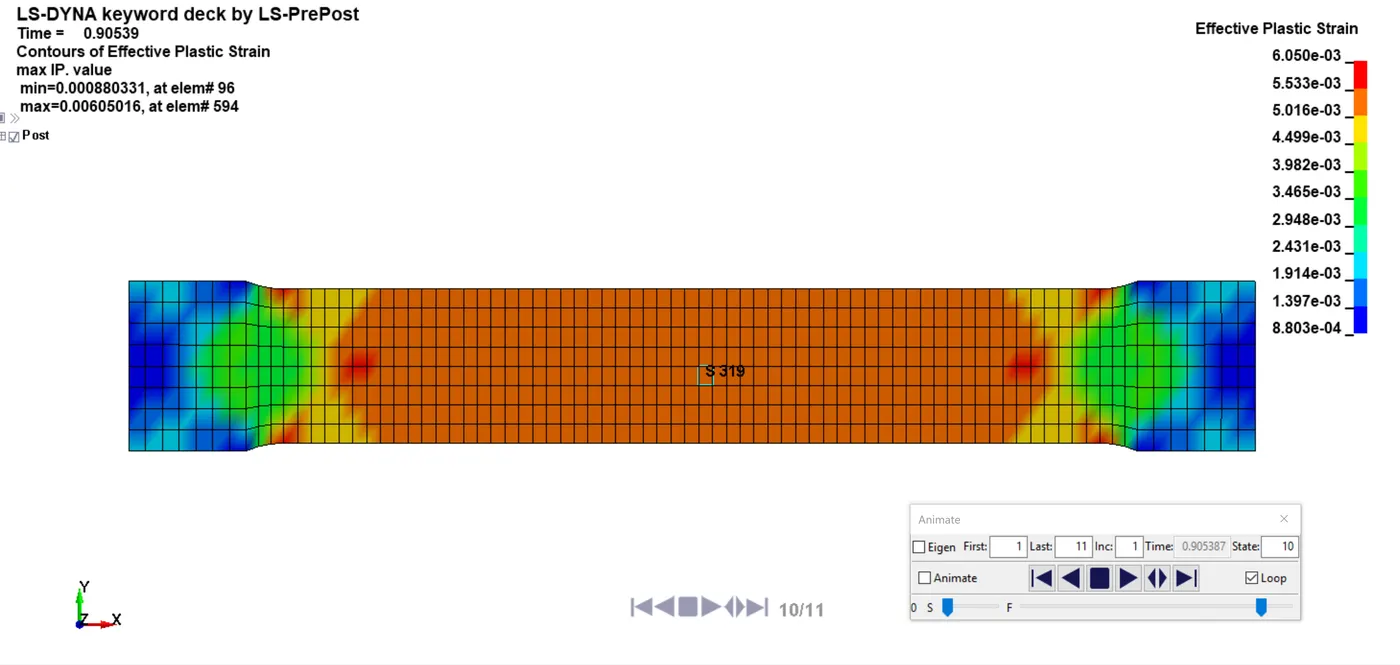
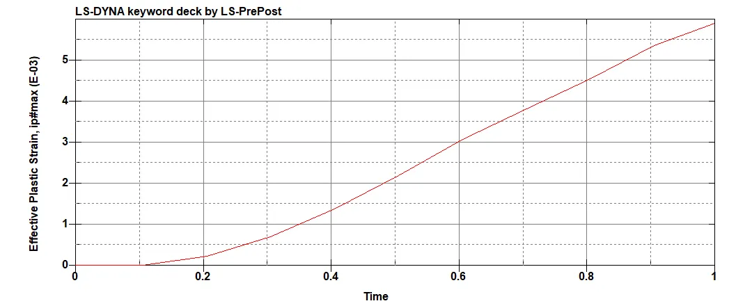
The maximum plastic strain in the model is observed to be 0.00605. This is seen in the below figure. The plastic strain keeps on increasing until the end of the simulation. This is expected given that the stress exceeds the yield stress value.

STRESS-STRAIN VALIDATION:

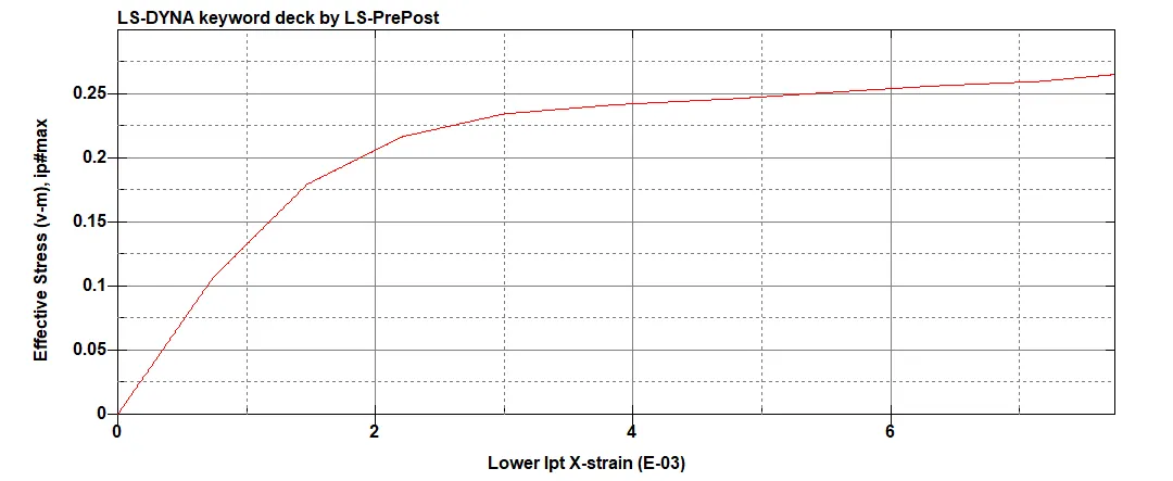
The curve obtained from LS PRE-POST is that of true strain vs tru stress. Hence this curve is compared to the true stress-true strain input curve and not effective stress vs strain curve. The material is stressed until it achieves 0.7% of its true strain value. No further hardening is taken into account. The simulation, as stated before is for low strain value. The combined stress-strain curve can be observed in the figure below:

CONCLUSION:

The given stress-strain curve has hence been validated using the MAT_024 plasticity card. Only the plastic portion of the curve has been considered for modeling and simulation.