Assignment 4

Objective:

• Run the model as it is. Name it as Law2_epsmax_failure.

• In FAIL/JOHNSON, change Ifail_sh=1, Dadv=1 & Ixfem=1. Run the model as Law2_epsmax_crack.

• Delete /Fail/JOHNSON card. Run the model as Law2_epsmax_nofail.

• Delete the value of Eps_p_max and the run the model with name Law2.

• Convert this material model into Law1 elastic with the same density, E, nu and run. Check the results.

• Open Law27_0000.rad.

• Check the shell properties and change it to recommended shell properties.

• Notice the material card. Johnson cook parameters but different values for EPS based failure.

• Run the model and name it as Law27

Compare 7 cases as discussed in last 3 slides, in a tabulated format on the basis of:

• The total number of cycles, Energy error, mass error and simulation time.

• Notice the animation of all 5 and describe the animations in brief on the
  basis of whether the elements are being deleted or cracked.

• Plot energies and notice any difference.

• Based on all the results, which case would represent the on-field
  scenario.

• Prepare a ppt/Docx and list down case by case result and your conclusion
  as to why the failure happened.

Procedure:

Case-1:

• Open the Hypermesh software and select the profile as "RADIOSS".

• Import the FAILURE_JOHNSON_0000.rad File by using the "Import Solverdeck" option present in the File menu at the top left of the window.

• After importing the file, run the model as it is without changing the properties.

• Click on the Analysis panel and select the Radioss tool in it.

• In the Input file select a folder to save the file by clicking on the Save as option.

• Change the file name as Law2_epsmax_failure and save the file.

• In the options enter the value as -nt 4 and click on the Radioss button to run the model.

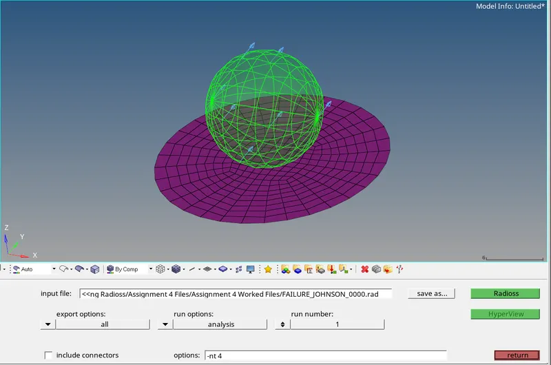
• Split the window into 2 layouts and open the HyperView in the 2nd window.

• Open the Law2_epsmax_failure.h3d file in the HyperView window and also check on the load results option in order to run the simulation.

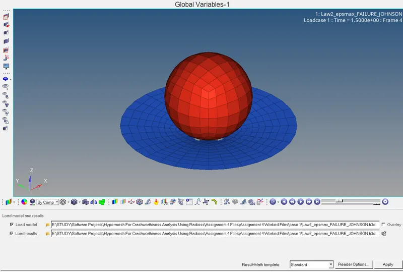
• Split the windows into another layout and open HyperGraph to plot the results.

• Open the Law2_epsmax_failure T01 file in the HyperGraph window and plot the Total energy, Hourglass energy, Contact energy, Internal energy & Total resultant force for the model.

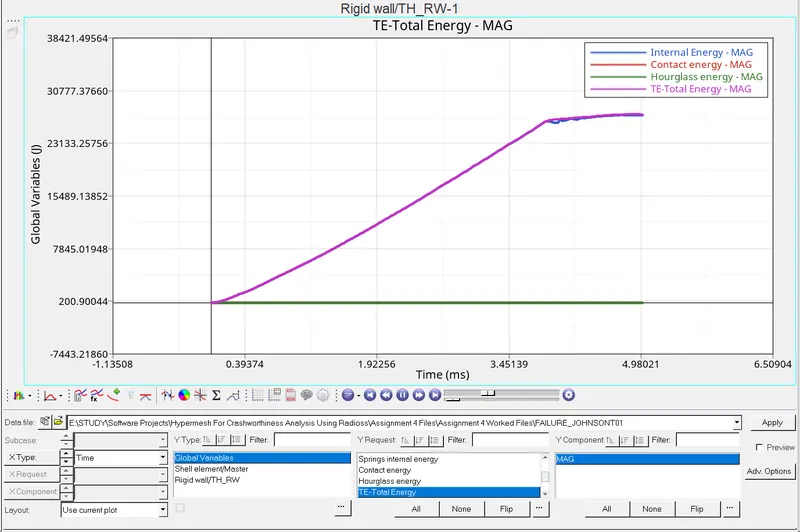
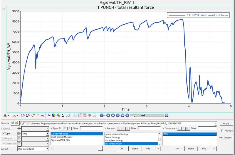
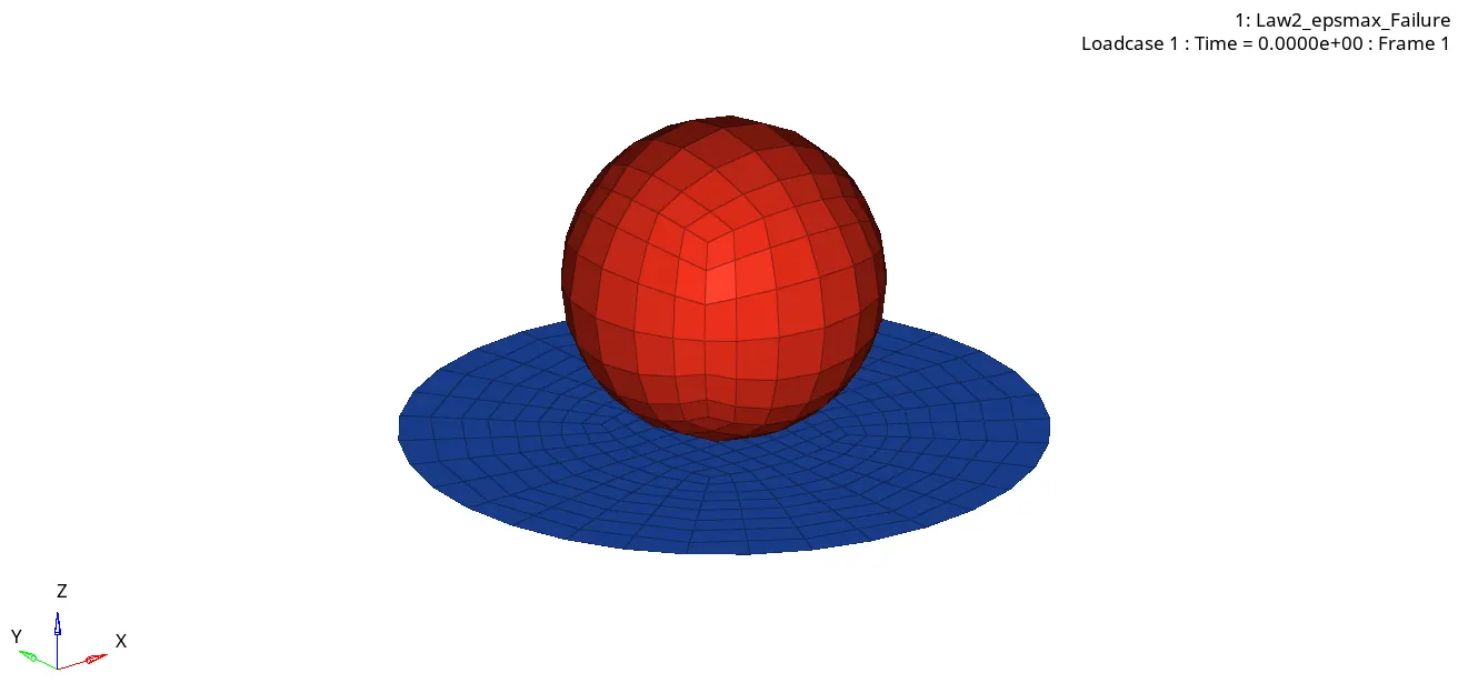
CASE 1 ANIMATION FILE

Case-2:

• After completing the case 1 use the same file and proceed onto the next case.

• Change the Ixfem, Dadv and Ifail_sh values to the recommended values in the Failure_johnson card and run the file.

• Click on the Analysis panel and select the Radioss tool in it.

• In the Input file select a folder to save the file by clicking on the Save as option.

• Change the file name as Law2_epsmax_crack and save the file.

• In the options enter the value as -nt 4 and click on the Radioss button to run the model.

• Split the window into 2 layouts and open the HyperView in the 2nd window.

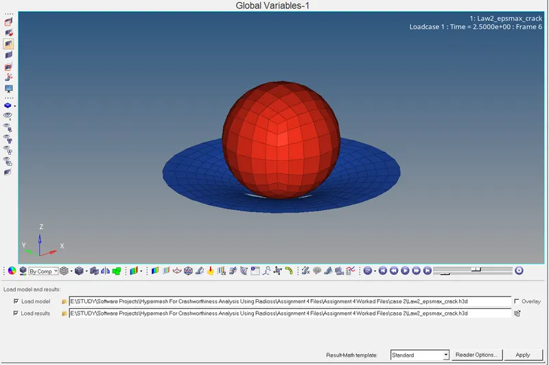
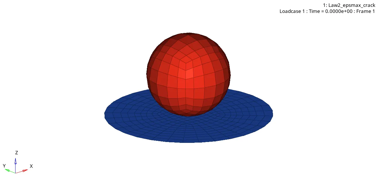
CASE 2 ANIMATION FILE

• Open the Law2_epsmax_crack.h3d file in the HyperView window and also check on the load results option in order to run the simulation.

• Split the windows into another layout and open HyperGraph to plot the results.

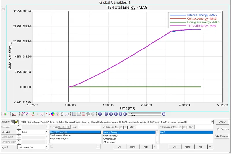
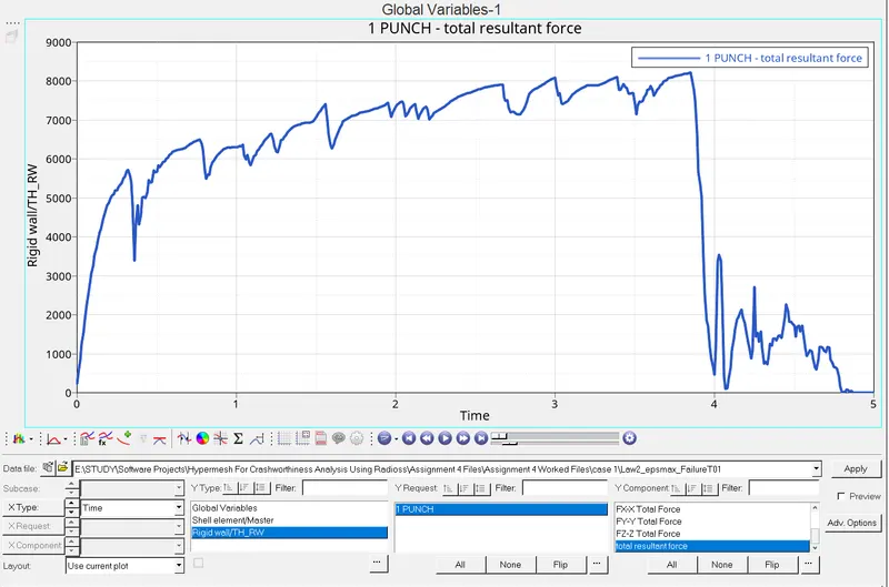
• Open the Law2_epsmax_crack T01 file in the HyperGraph window and plot the Total energy, Hourglass energy, Contact energy, Internal energy & Total resultant force for the model.

Case-3:

• Use the same file from case 2 to perform the case 3 analysis.

• Click on the Analysis panel and select the Radioss tool in it.

• In the Input file select a folder to save the file by clicking on the Save as option.

• Change the file name as Law2_epsmax_nofail and save the file.

• Delete the Failure_Johnson card in the solver browser and run the file.

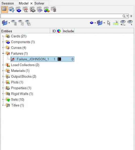
DELETING THE FAILURE JOHNSON CARD

• In the options enter the value as -nt 4 and click on the Radioss button to run the model.

• Split the window into 2 layouts and open the HyperView in the 2nd window.

• Open the Law2_epsmax_nofail.h3d file in the HyperView window and also check on the load results option in order to run the simulation.

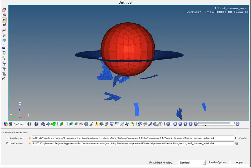
• Split the windows into another layout and open HyperGraph to plot the results.

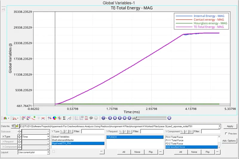
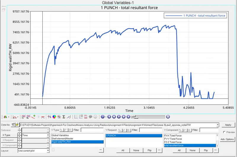
• Open the Law2_epspmax_nofail T01 file in the HyperGraph window and plot the Total energy, Hourglass energy, Contact energy, Internal energy & Total resultant force for the model.

Case-4:

• Use the same file from case 3 to perform the case 4 analysis.

• Click on the Analysis panel and select the Radioss tool in it.

• In the Input file select a folder to save the file by clicking on the Save as option.

• Delete the Eps_P_max value and make it as 0 in the material card and then run the file.

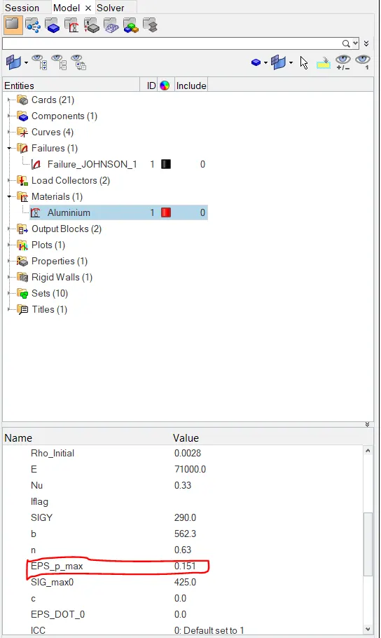
CHANGE THE EPS_p_max VALUE TO ZERO

• Change the file name as Law2 and save the file.

• In the options enter the value as -nt 4 and click on the Radioss button to run the model.

• Split the window into 2 layouts and open the HyperView in the 2nd window.

• Open the Law2 .h3d file in the HyperView window and also check on the load results option in order to run the simulation.

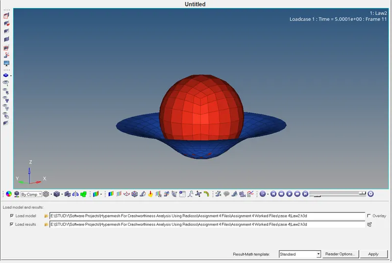
• Split the windows into another layout and open HyperGraph to plot the results.

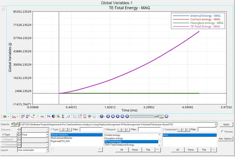
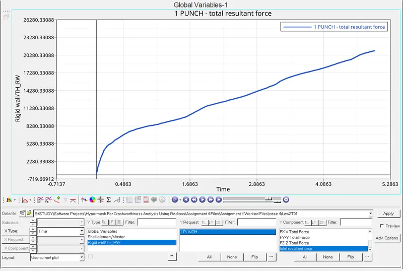
• Open the Law2 T01 file in the HyperGraph window and plot the Total energy, Hourglass energy, Contact energy, Internal energy & Total resultant force for the model.

Case-5:

• Use the same file from the case 4 to perform the case 5 analysis.

• In this case, change the material model to Law1 Elastic with the same Density, E, Nu in the material card and run.

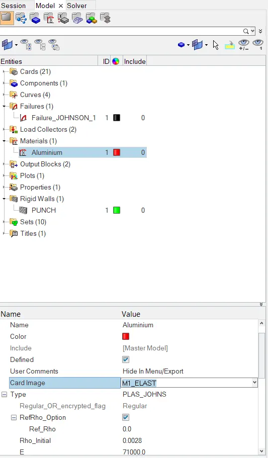
CHANGING THE MATERIAL MODEL IN THE MATERIAL CARD

• Click on the Analysis panel and select the Radioss tool in it.

• In the Input file select a folder to save the file by clicking on the Save as option.

• Change the file name as Law1_Elastic and save the file.

• In the options enter the value as -nt 4 and click on the Radioss button to run the model.

• Split the window into 2 layouts and open the HyperView in the 2nd window.

• Open the Law1_Elastic.h3d file in the HyperView window and also check on the load results option in order to run the simulation.

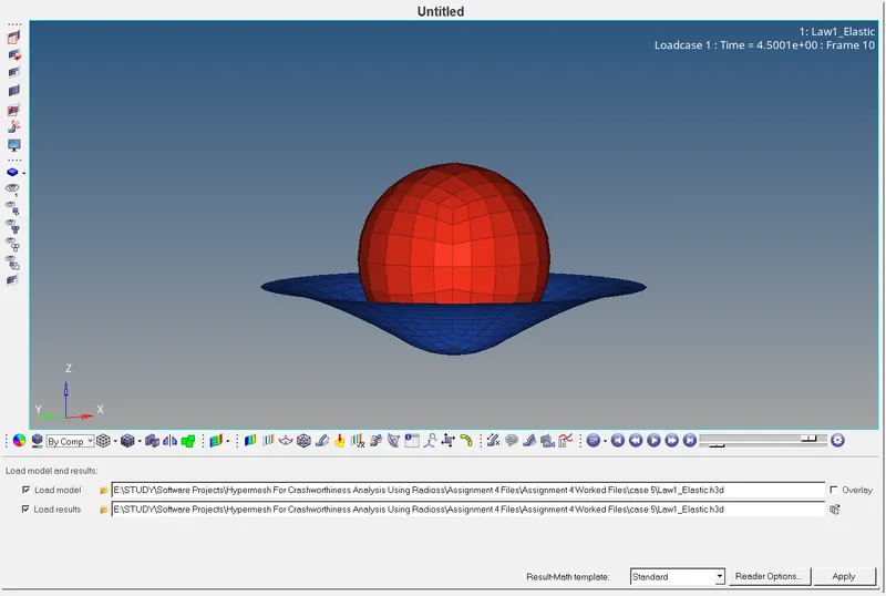
• Split the windows into another layout and open HyperGraph to plot the results.

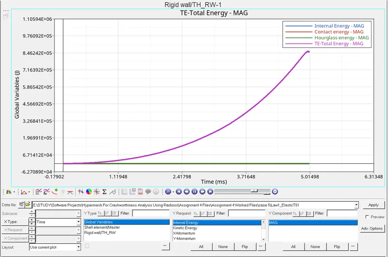
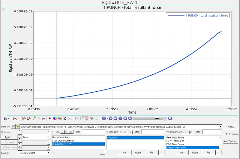
• Open the Law1_Elastic T01 file in the HyperGraph window and plot the Total energy, Hourglass energy, Contact energy, Internal energy & Total resultant force for the model.

Case-6:

• Open the Hypermesh software and select the profile as "RADIOSS".

• Import the Law_27_0000.rad File by using the "Import Solverdeck" option present in the File menu at the top left of the window.

• After importing the file, notice the properties and change the properties to the recommended properties and assign the property to the component.

• After assigning the property, click on the Analysis panel and select the Radioss tool in it.

• In the Input file select a folder to save the file by clicking on the Save as option.

• Change the file name as the Law_27 and save the file.

• In the options enter the value as -nt 4 and click on the Radioss button to run the model.

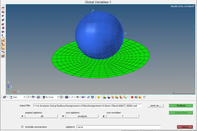
• Split the window into 2 layouts and open the HyperView in the 2nd window.

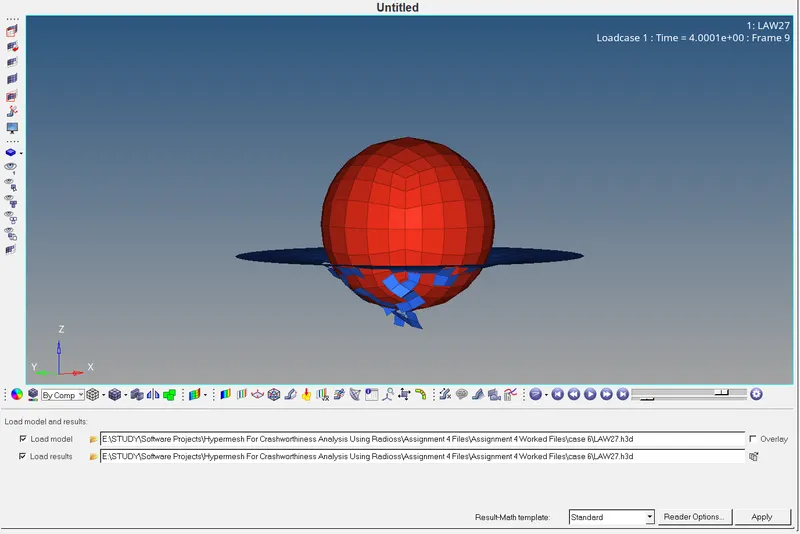
• Open the Law_27.h3d file in the HyperView window and also check on the Load results option in order to run the simulation.

• Split the windows into another layout and open HyperGraph to plot the results.

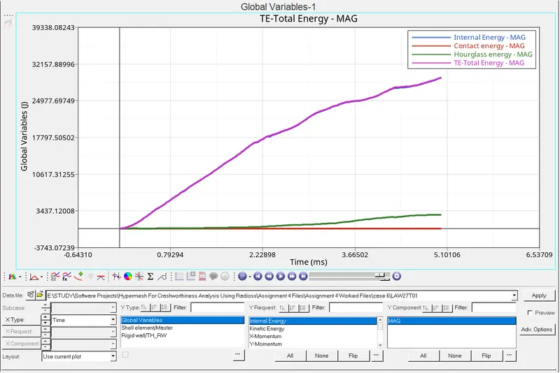
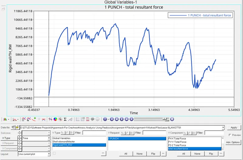
• Open the Law_27 T01 file in the HyperGraph window and plot the Total energy, Hourglass energy, Contact energy, Internal energy & Total resultant force for the model.

Case-7:

• Open the Hypermesh software and select the profile as "RADIOSS".

• Import the Failure_Johnson File by using the "Import Solverdeck" option present in the File menu at the top left of the window.

• After importing the file, notice the properties and change the properties to the recommended properties and assign the property to the component.

• Create a New curve according to the recommended parameters and name it as Test curve in the model tab.

• After creating the curve change the material model to Law36 in the material card and enter the values given in the Plas_tab card wherever necessary and assign the material to the component.

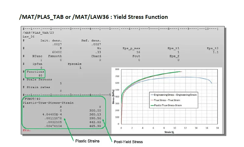
ENTER THE VALUES GIVEN IN THE LAW36 PLAS_TAB CARD

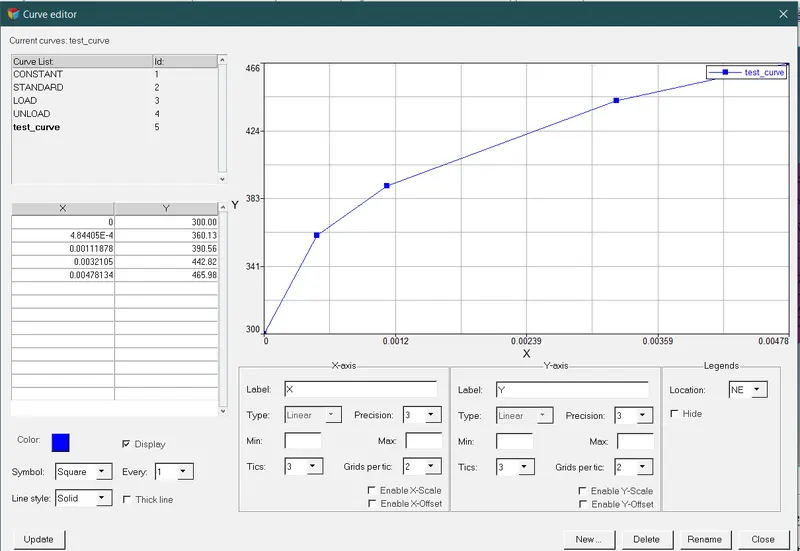
THE CURVE OBTAINED AFTER ENTERING THE GIVEN VALUES

• After assigning the property and material to the component, click on the Analysis panel and select the Radioss tool in it.In the Input file select a folder to save the file by clicking on the Save as option.

• Change the file name as the Law 36_Failure_Johnson and save the file.

• In the options enter the value as -nt 4 and click on the Radioss button to run the model.

• Split the window into 2 layouts and open the HyperView in the 2nd window.

• Open the Law_36 Failure_Johnson.h3d file in the HyperView window and also check on the Load results option in order to run the simulation.

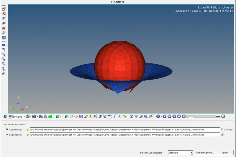
• Split the windows into another layout and open HyperGraph to plot the results.

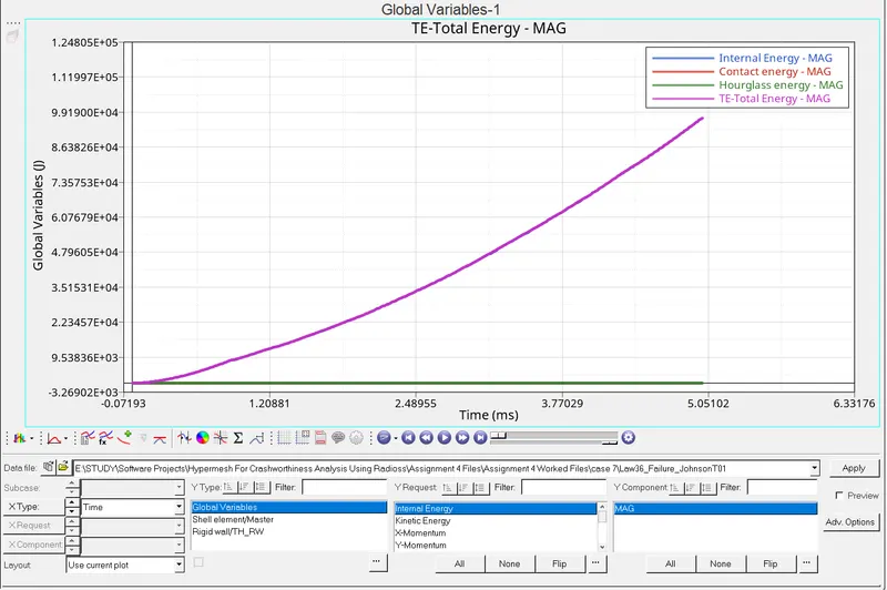
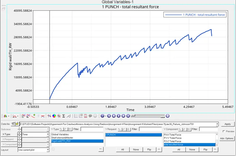
• Open the Law_36_Failure_Johnson T01 file in the HyperGraph window and plot the Total energy, Hourglass energy, Contact energy, Internal energy & Total resultant force for the model.

Comparison of all the cases:

.Out file data:

Cases Total no of cycles Energy error Mass error Simulation Time

1. Case-1 49479 + 0.2% 0.000 5.010
2. Case-2 49396 + 4.0% 0.000 5.010
3. Case-3 49404 + 0.8% 0.000 5.010
4. Case-4 48736 + 3.0% 0.000 5.010
5. Case-5 47968 + 0.3% 0.000 5.010
6. Case-6 41854 - 4.4 % 0.000 5.010
7. Case-7 53167 + 0.7% 0.000 5.010

Animation Comparison:

• Case 1: When the simulation is run in the given Recommended properties that are given with the model the elements get Deleted during the simulation.

• Case 2: After changing the values in the Failure Jhonson card in case 2 the elements also get Deleted during the simulation.

• Case 3: After deleting the Failure Jhonson card in case 3 the elements get Deleted during the simulation.

• Case 4: After deleting the Eps max value in the Material card in case 4 there is No rupture during the simulation.

• Case 5: After changing the material model to Law 1 Elastic with the same values in E, Nu & Density etc. There is No rupture taking place because of the elastic behaviour during the simulation.

• Case 6: In this case, the Law 27 file is used. The elements get Deleted during the simulation.

• Case 7: In this case, the Law 36 file is used. In this, the elements get Ruptured during the simulation.

Graph Comparison:

• The Hourglass energy and Contact energy have remained the same for all the cases except for the case 6.

• The Hourglass energy varies in the case of Law_27 file but the Contact energy remains the same.

• There is a steady increase in the Total energy & Internal energy at the start of the simulation and it stabilises just before the end for the first 3 Cases (i.e., Case 1, 2 & 3).

• There is a stable increase in the Total energy & Internal energy right from the start of the simulation and to the end for case 4, case 5, case 6 & case 7.

• The Rigid wall forces for case 1, case 2 and case 3 remain the same & for case 4, case 5, case 6 and case 7 remains different for each case.

On-field Scenario:

• The onfield scenario represents the case 7 because of the fact that it has an energy error of +0.7% which is acceptable when compared to other simulation in some cases because there is an acceptable limit of the positive value of 1%. If anything above 1% has to be checked because there is something going wrong in the simulation analysis.

• The Law_36 is most suitable for its elasto-plastic nature and it would be a preferred option.

• There is no mass error, no hourglass error and contact error.

Conclusion:

• The analysis has been performed for all the given cases.

• The graphs have been plotted for all the energies.

• The results have been tabulated and the energy error has been checked.

• Based on the results obtained from the onfield scenario the case 7 has been preferred.