Assignment 5

Objective:

• Create the mesh for bumper assembly, mesh size should be 6mm.

1. Run the crash tube model as it is.
2. Change the Inacti=6 and run.
3. Create the type 11 contact and run.
4. Remove both notches and remove boundary condition on rigid body node then run.
5. Create a new notch in the middle, select the whole section and run.
6. Create a new notch with nodes only from opposing 2 faces and run.

Note:

• Plot RWALL forces, contact forces, internal energy and Create TH/PART for all parts and compare results for all cases.
• Comment your thought on why there is a change in the internal energies.
• How does the notch affect the results?
• Plot energies and note any difference.

Bumper assembly procedure:

• Open the hypermesh software and select the profile as "RADIOSS".

• After that import the model by using the "Import model" option present in the file menu at the top.

• After importing the model, try to mesh the model by using the Automesh tool present in the 2D panel.

• Select the Automesh tool in the 2D panel, upon entering change the mesh type to mixed elements and enter the mesh value as 6mm.

• Select the surface of the component and click on the mesh button to generate the mesh on the selected surface.

• In the same way, try to mesh the remaining surfaces on the component.

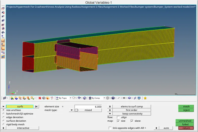
BUMPER ASSEMBLY MODEL WITH 6MM MESH

• After meshing the component, try to connect the individual surfaces with connectors.

• Select the connectors tool present in the 1D panel and select the spot tool to create a connection.

• Select the No of nodes on the surface in the nodes option and then select the components in the comps tool which are to be connected and enter the required tolerance value and in the type option

select the weld option to spot weld connection then click on the create button.

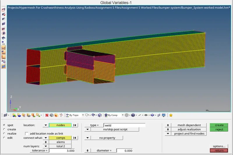
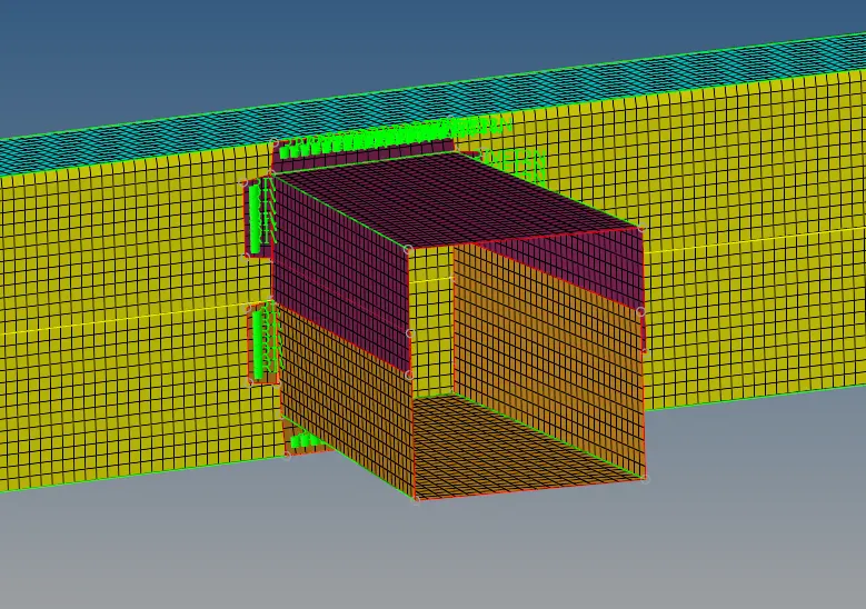
SPOTWELD CONNECTIONS

• Create the connectors wherever required to connect the individual components and save the model by using the save model option present in the file menu.

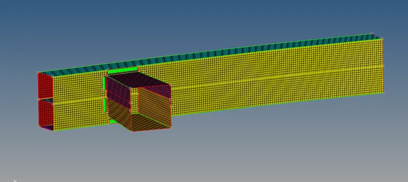
BUMPER ASSEMBLY MODEL FINAL MESH AND ALSO WITH SPOT WELD CONNECTIONS

Procedure for crush tube :

CASE 1:

• Open the hypermesh software and select the profile as "RADIOSS".

• After that import the model by using the "Import Solver Deck" option present in the file menu at the top.

• After importing the model click on the Radioss tool present in the Analysis panel.

• After importing the model, don't make any changes to the model run the file as it is which is mentioned for the case 1 file in the given question.

• In the Input file option, click on the save as option to change the file name and select the folder to save the model.

• Check on the Include connectors option and in the options enter the value as -nt 4 and click on the Radioss button to run the analysis.

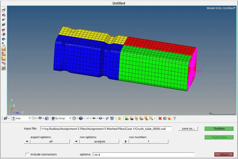
• After running the analysis, split the window into 3 layouts in order to open the Hyperview and HyperGraph.

• Both are the inbuilt applications within the HyperWorks software and both of them are used in order to review the results of the analysis at various time step intervals.

• Firstly open the Hyperview application, check on the load model and load results options and in the load model option click on the file icon and select & open the Crushtube.h3d file.

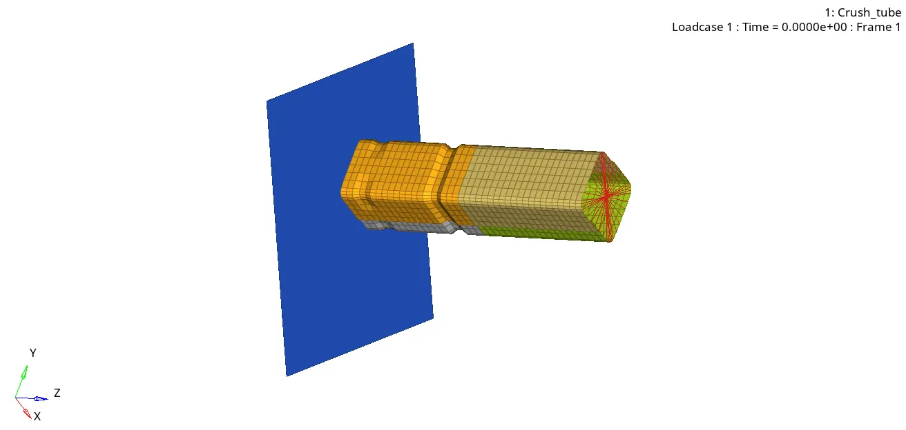
CASE 1 ANIMATION FILE

• After opening the Crushtube.h3d file, click on the Apply button present in the bottom corner in order to view the simulation.

• After looking at the simulation open the HyperGraph application in order to plot the Results of various energy parameters.

• Open the HyperGraph application, in the Data file option click on the file icon, select and open the CrushtubeT01 file present in the saved folder during the analysis in the hypermesh in order to plot the results.

• In the X type subcase select the Time, in the Y type subcase select the Global Variables, in the Y request select the Internal energy and in the Y component select the MAG option and then click on the apply button.

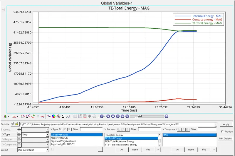
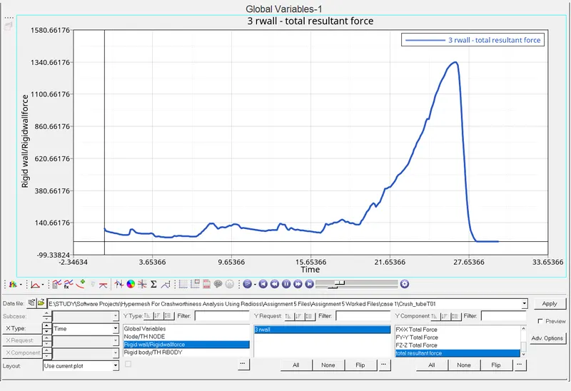
• Create the TH/PART for all the cases and run the file.

• In the same way, plot the remaining energy parameters for all the cases and compare the results.

CASE 2:

• In case 2 analysis, start working with case 1 file no need to import the given model again.

• Switch on the solver browser in the Model Tab select the INTER option in that select TYPE 7 and select the Self-contact in it.

• After selecting the Self-contact certain parameters are displayed in the status bar. Scroll down to the bottom and select the Inacti and change the value as 6.

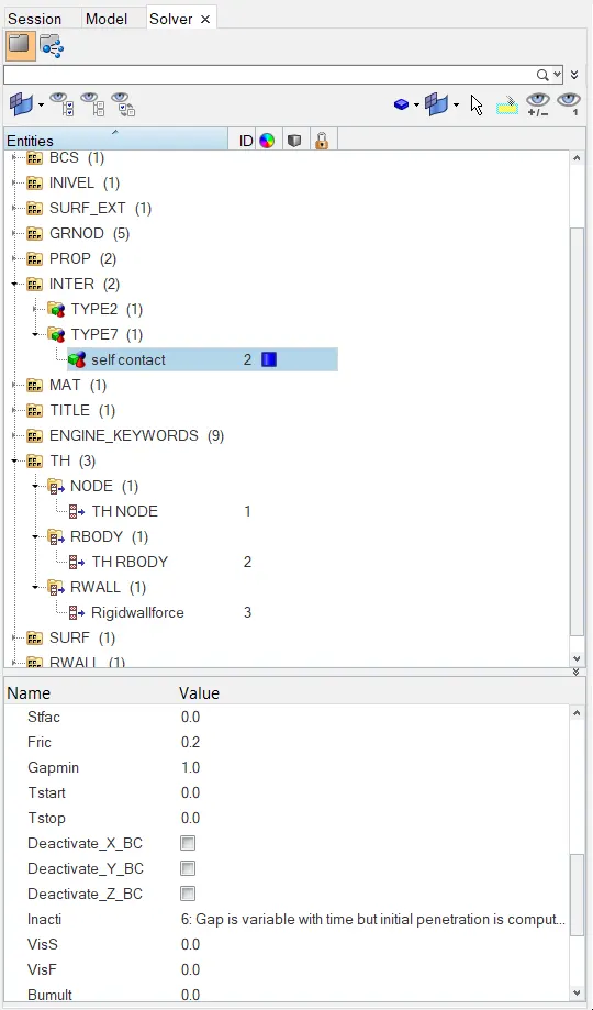
• After changing the value run the analysis and save it as case 2.

• In the Input file option, click on the save as option to change the file name and select the folder to save the model.

• Check on the Include connectors option and in the options enter the value as -nt 4 and click on the Radioss button to run the analysis.

• After running the analysis, split the window into 3 layouts in order to open the Hyperview and HyperGraph.

• Both are the inbuilt applications within the HyperWorks software and both of them are used in order to review the results of the analysis at various time step intervals.

• Firstly open the Hyperview application, check on the load model and load results options and in the load model option click on the file icon and select & open the Crushtube.h3d file.

• After opening the Crushtube.h3d file, click on the Apply button present in the bottom corner in order to view the simulation.

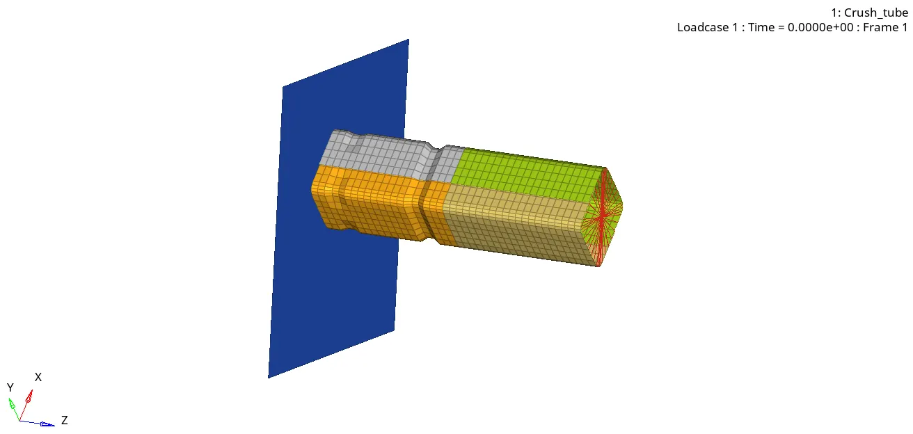
CASE 2 ANIMATION FILE

• After looking at the simulation open the HyperGraph application in order to plot the Results of various energy parameters.

• Open the HyperGraph application, in the Data file option click on the file icon, select and open the CrushtubeT01 file present in the saved folder during the analysis in the hypermesh in order to plot the results.

• In the X type subcase select the Time, in the Y type subcase select the Global Variables, in the Y request select the Internal energy and in the Y component select the MAG option and then click on the apply button.

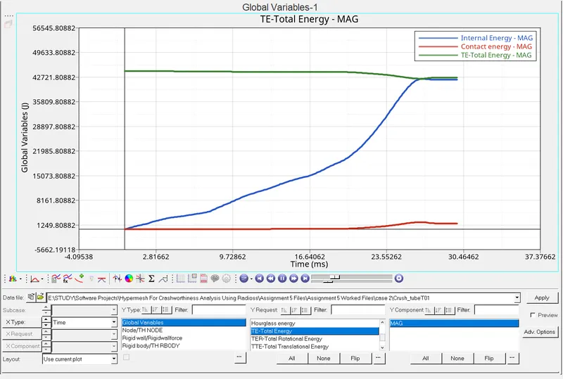
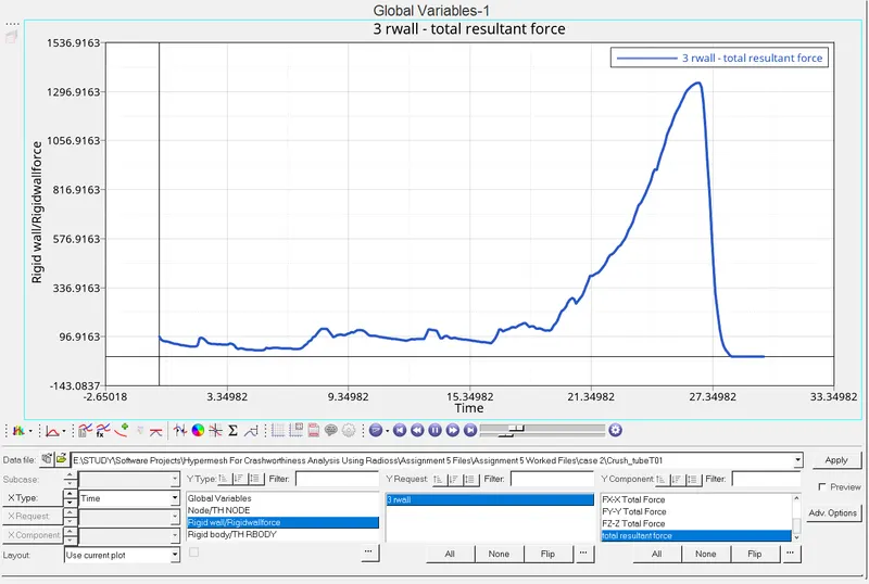
• Create the TH/PART for all the cases and run the file.

• In the same way, plot the remaining energy parameters for all the cases and compare the results.

CASE 3:

• In case 3 analysis, start working with case 2 file no need to import the given model again.

• Click on the Solver browser in the tab area then Right-click and select the create option and select INTER option and select the TYPE 11 CONTACT in it.

• The TYPE11 CONTACT is displayed along with the existing TYPE 7 and TYPE 2 contact in the INTER tool in the solver browser.

• Click on the TYPE11 CONTACT (EDGE TO EDGE CONTACT) and enter the values for certain parameters and select the master and slave in the status bar.

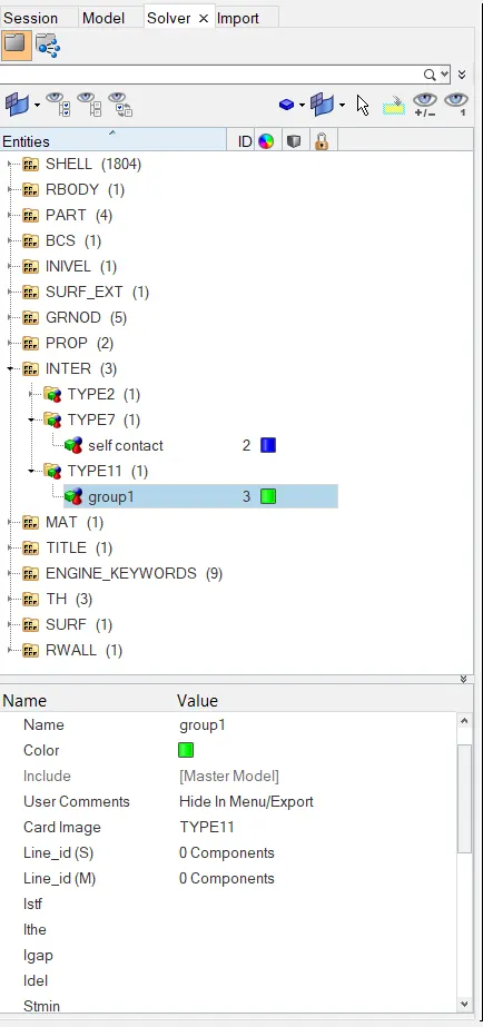
• In the Input file option, click on the save as option to change the file name and select the folder to save the model.

• Check on the Include connectors option and in the options enter the value as -nt 4 and click on the Radioss button to run the analysis.

• After running the analysis, split the window into 3 layouts in order to open the Hyperview and HyperGraph.

• Both are the inbuilt applications within the HyperWorks software and both of them are used in order to review the results of the analysis at various time step intervals.

• Firstly open the Hyperview application, check on the load model and load results options and in the load model option click on the file icon and select & open the Crushtube.h3d file.

• After opening the Crushtube.h3d file, click on the Apply button present in the bottom corner in order to view the simulation.

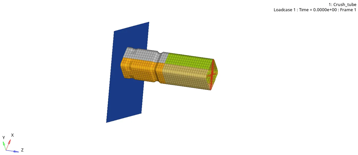
CASE 3 ANIMATION FILE

• After looking at the simulation open the HyperGraph application in order to plot the Results of various energy parameters.

• Open the HyperGraph application, in the Data file option click on the file icon, select and open the CrushtubeT01 file present in the saved folder during the analysis in the hypermesh in order to plot the results.

• In the X type subcase select the Time, in the Y type subcase select the Global Variables, in the Y request select the Internal energy and in the Y component select the MAG option and then click on the apply button.

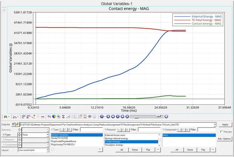
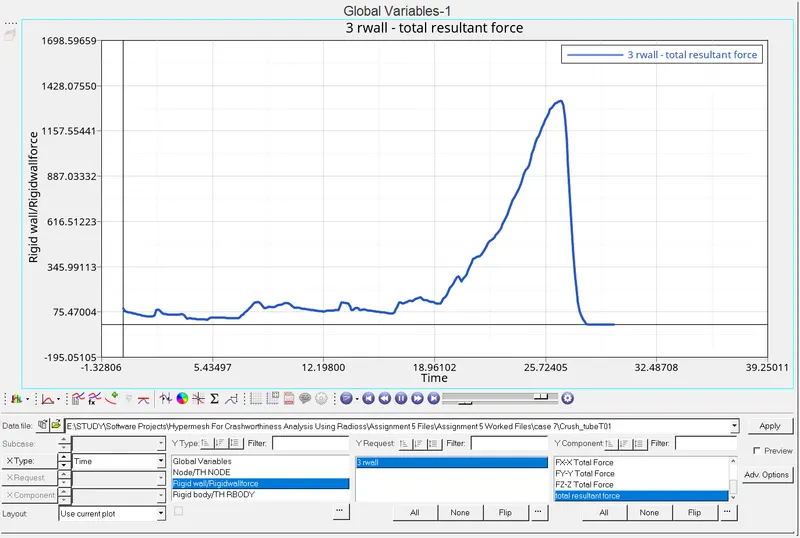
• Create the TH/PART for all the cases and run the file.

• In the same way, plot the remaining energy parameters for all the cases and compare the results.

CASE 4 :

• In case 4 analysis, start working with case 3 file no need to import the given model again.

• In this case, we need to remove the existing boundary conditions on the rigid body and also the notches on the component.

• Click on the solver browser and select the boundary conditions in it and remove the boundary conditions card.

• After removing the boundary conditions try to remove the notches on the component on both sides by using the Align node or F7 tool present in the geometry panel.

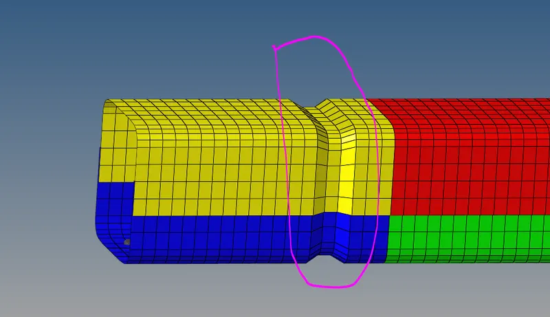
THE COMPONENT BEFORE REMOVING NOTCHES

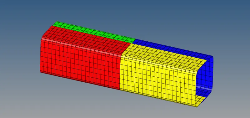
COMPONENT AFTER REMOVING ALL NOTCHES

• After removing the notches try to run the model for analysis.

• In the Input file option, click on the save as option to change the file name and select the folder to save the model.

• Check on the Include connectors option and in the options enter the value as -nt 4 and click on the Radioss button to run the analysis.

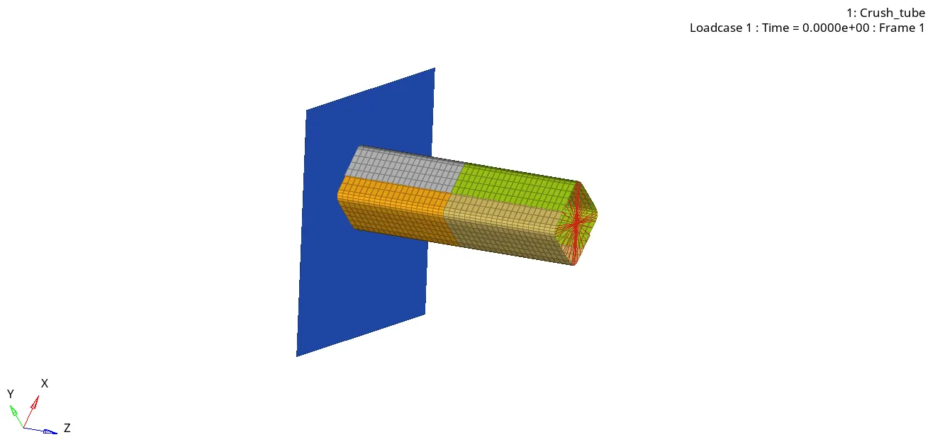
CASE 4 ANIMATION FILE

• After running the analysis, split the window into 3 layouts in order to open the Hyperview and HyperGraph.

• Both are the inbuilt applications within the HyperWorks software and both of them are used in order to review the results of the analysis at various time step intervals.

• Firstly open the Hyperview application, check on the load model and load results options and in the load model option click on the file icon and select & open the Crushtube.h3d file.

• After opening the Crushtube.h3d file, click on the Apply button present in the bottom corner in order to view the simulation.

• After looking at the simulation open the HyperGraph application in order to plot the Results of various energy parameters.

• Open the HyperGraph application, in the Data file option click on the file icon, select and open the CrushtubeT01 file present in the saved folder during the analysis in the hypermesh in order to plot the results.

• In the X type subcase select the Time, in the Y type subcase select the Global Variables, in the Y request select the Internal energy and in the Y component select the MAG option and then click on the apply button.

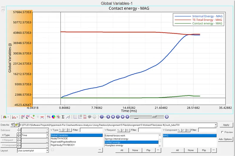
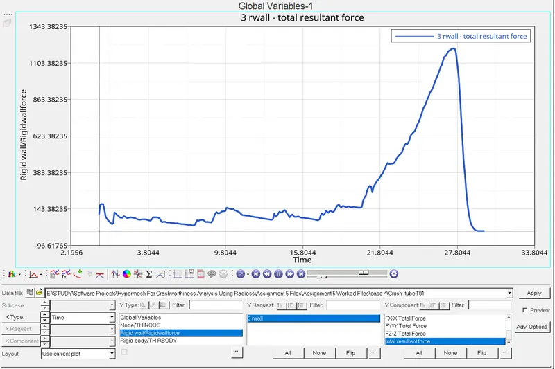
• Create the TH/PART for all the cases and run the file.

• In the same way, plot the remaining energy parameters for all the cases and compare the results.

CASE 5:

• In case 5 analysis, start working with the case 4 analysis model no need to import the model again.

• For case 5 analysis, create a new notch in the middle for the model parts.

• To create a new notch in the middle use the translate tool present in the tool panel in the hypermesh.

• After creating the new notch in the middle try to run the model by using the Radioss tool in the Analysis panel.

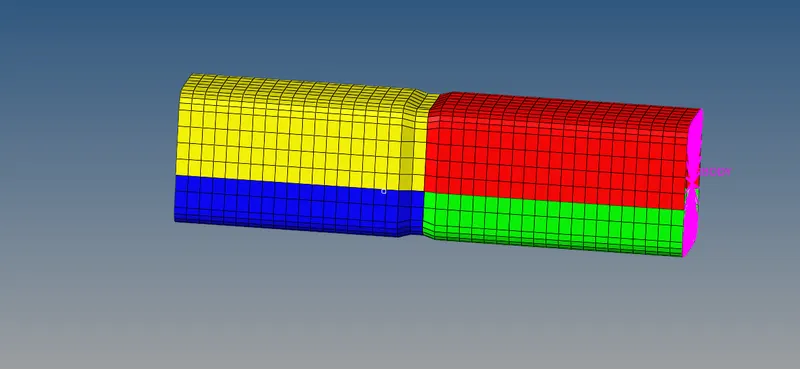
AFTER CREATING A NEW NOTCH IN THE MIDDLE USING THE TRANSLATE TOOL

• In the Input file option, click on the save as option to change the file name and select the folder to save the model.

• Check on the Include connectors option and in the options enter the value as -nt 4 and click on the Radioss button to run the analysis.

• After running the analysis, split the window into 3 layouts in order to open the Hyperview and HyperGraph.

• Both are the inbuilt applications within the HyperWorks software and both of them are used in order to review the results of the analysis at various time step intervals.

• Firstly open the Hyperview application, check on the load model and load results options and in the load model option click on the file icon and select & open the Crushtube.h3d file.

• After opening the Crushtube.h3d file, click on the Apply button present in the bottom corner in order to view the simulation.

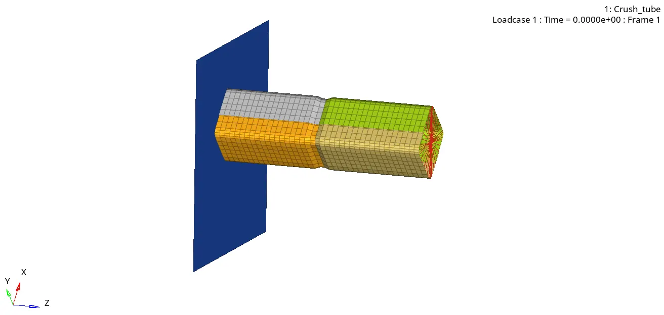
CASE 5 ANIMATION FILE

• After looking at the simulation open the HyperGraph application in order to plot the Results of various energy parameters.

• Open the HyperGraph application, in the Data file option click on the file icon, select and open the CrushtubeT01 file present in the saved folder during the analysis in the hypermesh in order to plot the results.

• In the X type subcase select the Time, in the Y type subcase select the Global Variables, in the Y request select the Internal energy and in the Y component select the MAG option and then click on the apply button.

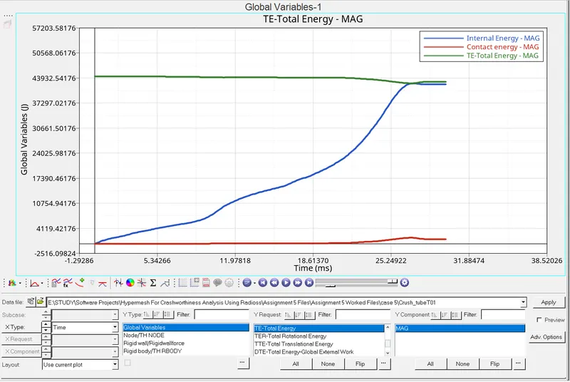
• Create the TH/PART for all the cases and run the file.

• In the same way, plot the remaining energy parameters for all the cases and compare the results.

CASE 6:

• In case 6 analysis, start working with the case 5 analysis model no need to import the model again.

• For case 6 analysis, create a new notch anywhere on the component on the opposite faces for the model parts.

• To create a new notch in the opposite faces use the translate tool present in the tool panel in the hypermesh.

• After creating the new notch in the opposite faces try to run the model by using the Radioss tool in the Analysis panel.

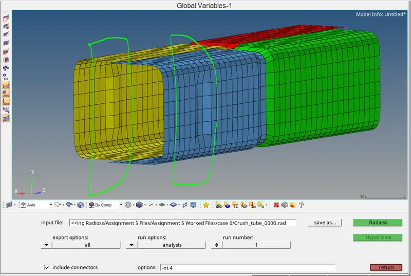
CASE 6 MODEL WITH NOTCHES ON THE OPPOSITE FACES

• In the Input file option, click on the save as option to change the file name and select the folder to save the model.

• Check on the Include connectors option and in the options enter the value as -nt 4 and click on the Radioss button to run the analysis.

• After running the analysis, split the window into 3 layouts in order to open the Hyperview and HyperGraph.

• Both are the inbuilt applications within the HyperWorks software and both of them are used in order to review the results of the analysis at various time step intervals.

• Firstly open the Hyperview application, check on the load model and load results options and in the load model option click on the file icon and select & open the Crushtube.h3d file.

• After opening the Crushtube.h3d file, click on the Apply button present in the bottom corner in order to view the simulation.

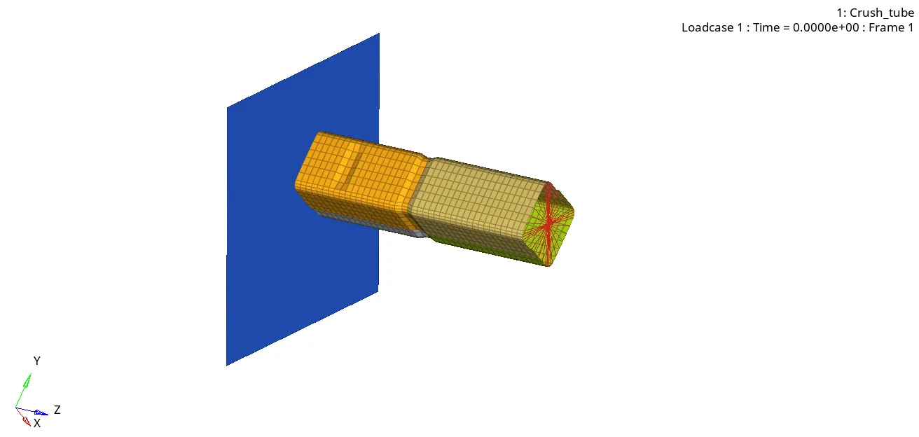
CASE 6 ANIMATION FILE

• After looking at the simulation open the HyperGraph application in order to plot the Results of various energy parameters.

• Open the HyperGraph application, in the Data file option click on the file icon, select and open the CrushtubeT01 file present in the saved folder during the analysis in the hypermesh in order to plot the results.

• In the X type subcase select the Time, in the Y type subcase select the Global Variables, in the Y request select the Internal energy and in the Y component select the MAG option and then click on the apply button.

• Create the TH/PART for all the cases and run the file.

• In the same way, plot the remaining energy parameters for all the cases and compare the results.

Comparison of all cases:

Case 1:

• For the 1st case when the simulation starts, the internal energy rises gradually from the start of the simulation and stabilizes once it reaches 42500 J at 25-30 ms.

• The Rigid wall force attains a value of 1340 N during the simulation for case 1.

• Contact energy remains the same throughout the simulation. The mass error is 0.000 and the energy error is -3.8%.

Case 2:

• For the 2nd case after changing the inacti value as 6 the internal energy value increases gradually from the start and stabilizes once it reaches up to 42500 J at the 25-30 ms. There is a decrease in

the internal energy value compared to the 42500 in case 1 after changing the inacti value from 0 to 6.

• The Rigid wall force attains a value of 1300 N during the simulation for case 2.

• Contact energy remains the same throughout the simulation. The mass error is 0.000 and the energy error is -3.8%.

Case 3:

• For the 3rd case, the Type 11 contact (edge to edge contact) had been introduced. The internal energy increases gradually from the start and it stabilizes at 42500 J at the end of the simulation at 25-

30 ms.

• The Rigid wall force attains a value of 1300 N during the simulation for case 3.

• Contact energy remains the same throughout the simulation. The mass error is 0.000 and the energy error is -3.8%.

Case 4:

• For the 4rth case, the notches have been removed on both sides and the existing boundary conditions on the rigid body. The internal energy increases gradually at the start of the simulation and stabilizes

at 42000 J in the end at 25-30 ms.

• The Rigid wall force attains a value of 1250 N during the simulation for the case 4.

• Contact energy remains the same throughout the simulation. The mass error is 0.000 and the energy error is -3.1%.

Case 5:

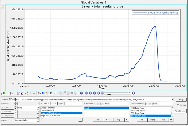
• For the 5th case, after creating a notch in the middle. The internal energy increases gradually at the start of the simulation and stabilizes at 42500 J in the end at 25-30 ms.

• The Rigid wall force attains a value of 1400 N during the simulation for case 5.

• Contact energy remains the same throughout the simulation. The mass error is 0.000 and the energy error is -2.9%.

Case 6:

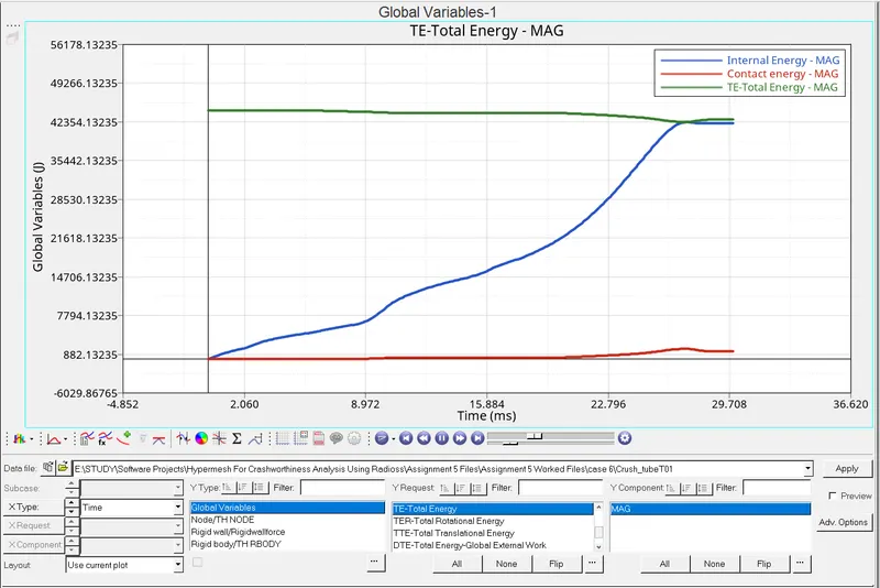
• For the 6th case, after creating the notch in the opposite faces on the component. The internal energy increases gradually at the start of the simulation and stabilizes at 42500 J in the end at 25 - 30

ms.

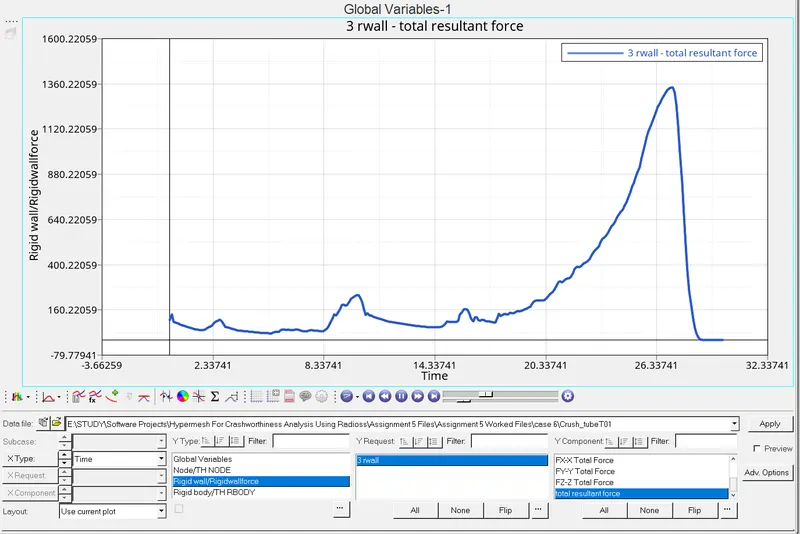
• The Rigid wall force attains a value of 1340 N during the simulation for the case 6.

• Contact energy remains the same throughout the simulation. The mass error is 0.000 and the energy error is -3.2%.

Energy Comparison:

• During the simulation, the rigid wall force attains a peak value of 1400 N this happens in the 5th case and rest of all the cases but the lowest was at case 4 where there is no notch the rigid wall force

the value during this case recorded as 1250N.

• The contact energy remains pretty much the same for all cases with little changes at the top.

• The internal energy value remains the same for all the cases when the graphs are plotted where there are notches present in the model except for case 4 where there is a very small decrease in the internal energy in case 4 where there is no notch present in the model.

Notch Comparison:

• When there is no notch in case 4 the crushing of the tube takes place uniformly compared to the rest of the cases because of no notches present in the model.

• When the notch present in 2 opp sides in case 6 the sides are subjected to deformation when the start of the simulation and rest of the component deformation takes place.

• The stress concentration is more near the area where notch present and there is a chance that the component might deform due to less force but notches also help in determine the strain formation.

if notches are not present then it is not possible to determine the strain formation that's what happened in case 4.

Conclusion:

• The bumper assembly has meshed with 6mm and the connections have been created.

• The Rigid wall forces, contact forces and internal energy have been plotted.

• The TH/Part for all parts has been created.

• The difference in the internal energy and the notch effect is explained.

• The energy difference has been noted and they are compared.