SIMULATION OF TRANSIENT BEHAVIOUR OF A SIMPLE PENDULUM

AIM :

To simulate the transient behaviour of a simple pendulum and to create an animation of it's motion.

TOOLS REQUIRED :

MATLAB

THEORY :

Simple Pendulum

A simple pendulum consists of a mass m hanging from a string of length L and fixed at a pivot point P. When displaced to an initial angle and released, the pendulum will swing back and forth with periodic motion. By applying Newton's secont law for rotational systems, the equation of motion for the pendulum may be obtained.

`(d^2theta)/dt^2+b/m((d theta)/dt)+g/Lsintheta=0`

where,

`theta` = Instantaneous angular displacement

t = time

b = Damping co-efficient

m = mass

g = acceleration due to gravity (9.81 `m/s^2`)

L = length of pendulum

This is the equation of motion of a simple pendulum with damping.

Ordinary Differential Equation (ODE)

In mathematics, an ordinary differential equation (ODE) is a differential equation containing one or more functions of one independent variable and the derivatives of those functions. The term ordinary is used in contrast with the term partial differential equation which may be with respect to more than one independent variable. Some ODEs can be solved explicitly in terms of known functions and integrals. When that is not possible, the equation for computing the Taylor series of the solutions may be useful. For applied problems, numerical methods of ordinary differential equations can supply an approximation of the solution.

A simple example is Newton's second law of motion — the relationship between the displacement x and the time t of an object under the force F, is given by the differential equation

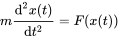
which constrains the motion of a particle of constant mass m.

In general, F is a function of the position x(t) of the particle at time t. The unknown function x(t) appears on both sides of the differential equation, and is indicated in the notation F(x(t)).

PROGRAM CODE :

Main program to solve the second order differential equation of simple pendulum

clear all
close all
clc

b = 0.05;
g = 9.81;
l = 1;
m = 0.1;

%initial conditions
theta_0 = [0;3];

%time points
t_span = linspace(0,20,500);

%solving ODE
[t results] = ode45(@(t,theta) ode_func(t,theta,b,g,l,m),t_span,theta_0);

%plotting
plot(t,results(:,1),'color','r')
hold on
plot(t,results(:,2),'color','b')
xlabel('Time')
ylabel('Plot')
legend('Angular Displacement','Angular Velocity')

ct = 1;
for i = 1:length(t_span)
    x0 = 0;
    y0 = 0;
    x1 = l*sind(results(i,1));
    y1 = -l*cosd(results(i,1));
    figure(2)
    plot([-0.05 0.05],[0 0],'linewidth',10,'color','g')
    hold on
    plot([x0 x1],[y0 y1],'linewidth',3,'color','b')
    axis([-0.1 0.1 -2 1])
    hold on
    plot(x1,y1,'marker','o','markersize',20,'markerfacecolor','r')
    pause(0.003)
    M(ct) = getframe(gcf);
    hold off
    ct=ct+1;
end

figure()
movie(M)
videofile = VideoWriter('Simple Pendulum.avi','Uncompressed AVI');
open(videofile)
writeVideo(videofile,M)
close(videofile)

User-defined function to transform 2nd order DE into two 1st order DE

function [dtheta_dt] = ode_func(t,theta,b,g,l,m)
theta1 = theta(1)
theta2 = theta(2)
dtheta1_dt = theta2;
dtheta2_dt = -(b/m)*theta2 - (g/l)*sin(theta1);
dtheta_dt = [dtheta1_dt;dtheta2_dt];
end

Code Explanation

1. First, the input parameters such as b,g,m and l are initialized with the given values.
2. The initial boundary condition i.e., the displacement and velocity at time t=0 is initialized into a column array named 'theta_0'.
3. An array named 't_span' is initialized to store the time points at which we want to plot the displacement and velocity graphs.
4. In this step, the 2nd order differential equation is solved by calling the in-built function "ode45()" . This function takes in 2nd order differential equation to solve and return the output. But the equation we need to solve is a 2nd order differential equation.

So, we have to define a function ode_func() to transform the 2nd order differential equation into two1st order differential equation.

The transformation equations are given below :

Let `theta=theta1`

`therefore (d theta)/dt = (d theta1)/dt = theta2` .........(1)

Also, `(d^2 theta)/dt^2=(d^2 theta1)/dt^2=d/dt((d theta1)/dt)=(d theta2)/dt` ........(2)

Putting (1) and (2) in the differential equation of simple pendulum,

`(d theta2)/dt+b/mtheta2+g/Lsintheta1=0`

Therefore, `(d theta1)/dt = theta2` and `(d theta2)/dt=-b/mtheta2-g/Lsintheta1`

`d/dt[theta1;theta2] =[theta2;-b/mtheta2-g/Lsintheta1]`

`d/dt[theta1;theta2]` is the solution vector.

V. The ode45() function solves the two 1st order differential equations returned by the function ode_func() using the following command

[t results] = ode45(@(t,theta) ode_func(t,theta,b,g,l,m),t_span,theta_0);

RESULTS :

• Plot of angular displacement and angular velocity with respect to time

• Animation of the simple pendulum

CONCLUSIONS :

The transient behaviour of a simple pendulum is simulated using MATLAB and an animation video is created.

Link to animation video on YouTube : https://youtu.be/AvPEMDFGQus