Week - 10 Hyperelastic Material Models

AIM :

       To model a Hyperelastic material using *MAT_HYPERELASTIC_RUBBER (077_H) and *MAT_OGDEN_RUBBER (077_O) material models from the given Eng. Stress-Strain data and verify the models by conducting a tensile test simulation on the Dog-Bone specimen.

TOOLS REQUIRED :

• LS-PrePost
• LS-Run
• MS-Excel

INTRODUCTION :

       Hyperelastic materials are the special class of materials which respond elastically even when they are subjected to large deformations. They show both a nonlinear material behavior as well as large shape changes. They are characterized by:

1. Can undergo large elastic deformations in order of 100 to 700% which are fully recoverable, i.e., the initial shape is recovered when load is removed.
2. Are nearly incompressible, which means that they change can their shape but overall volume remains almost constant.
3. Show a highly nonlinear stress-strain relation.
4. The material softens and then becomes stiffer again when applied to tension whereas, under compression, they have a quite stiff response.

Many polymers show hyperelastic behavior, such as elastomers, rubbers, and other similar soft flexible materials.

       Hyperelastic materials are mostly used in applications where high flexibility, in the long run, is required, under the presence of high loads. Some typical examples of their use are as elastomeric pads in bridges, rail pads, car door seal, car tires, and fluid seals.

       Hyperelastic materials use something called a strain energy density function to derive the relationship between stress and strain. This allows them to model the relationship between stress and strain accurately even when the strain is between 100% to 700%, depending on the exact hyperelastic model that is used.

                                                                                 

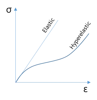
                                                                       Difference between a Hyperelastic material and an Elastic material

       In finite element analysis, the hyperelasticity theory is used to represent the non-linear response of hyperelastic materials at large deformations. Hyperelasticity is popular due to its ease of use in finite element models. Usually, stress-strain curve data from experimental tests is used to fit the constants of theoretical models, thus approximating the material response.

LS-DYNA offers mainly 4 kinds of hyperelastic material models as below.

1. Neo-Hookean : Fastest, Strains up to 100%, Most accurate for Uniaxial strain
2. Mooney-Rivlin : Slower than Neo-Hooke, Strains up to 200%, often the most popular
3. Ogden : Slowest, Strains up to 700%, Very general purpose hyperelastic material model
4. Arruda-Boyce : Slower than Mooney-Rivlin, Strains up to 300%, Special purpose hyperelastic material for certain rubbery materials such as silicon and neoprene

PROCEDURE :

NOTE : (g,mm,ms) unit system is followed consistently throughout the whole study.

• The material data for which the material model has to created is shown below.

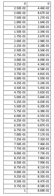
• The given data is the Engineering Stress-Strain data in [MPa/(mm/mm)].
• The data is imported into Excel and plotted as shown below.

 

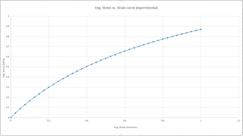
                                                                   Experimental Eng. Stress-Strain data plot

• Now, the Dog-Bone specimen is opened in LS-PrePost.

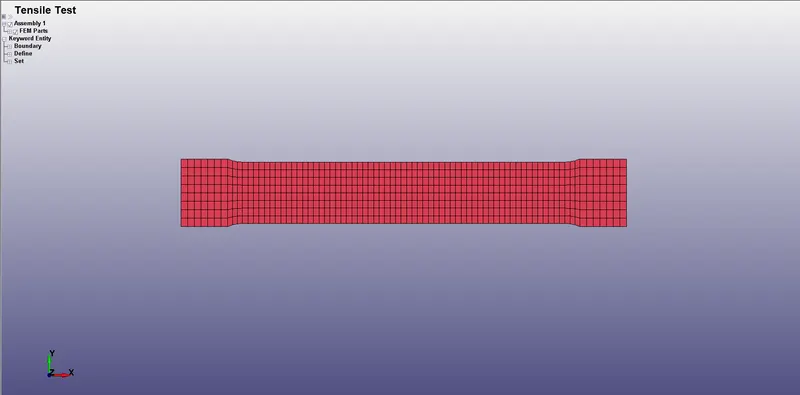
                                                                                                             Dog-Bone 2D specimen

• The section properties for the Dog-Bone are defined by using *SECTION_SHELL keyword. All the properties are set to default and a thickness of 2.67mm is assigned to the shell elements.

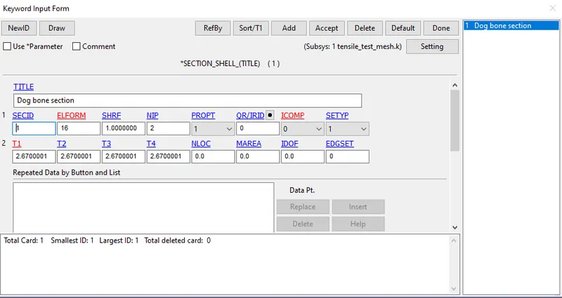
                                                               Section definition for the Dog-Bone part

• The Eng. Stress-Strain data is input as a curve using *DEFINE_CURVE keyword as shown below.

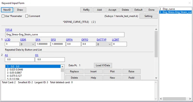
                                                                       Defining Eng. Stress-Strain curve

• Material for the specimen is modelled using two different material model cards separately.
  
  • *MAT_HYPERELASTIC_RUBBER (077_H)
  • *MAT_OGDEN_RUBBER (077_O)

• In the first case, material is modelled using *MAT_HYPERELASTIC_RUBBER (077_H) model.
• Parameters such as density, Poisson's ratio, number of constants to solve for (N) are input in the material card.
• The parameter N determines the order of the polynomial with which the Strain Energy-Stretch curve is to be fitted.
• Initially, the curve is fitted with a ploynomial of order 1, i.e., N is set to 1.
• The defined Eng. Stress-Strain curve is given as input for the Strain Energy-Stretch curve fitting, through LCID1 parameter.

 

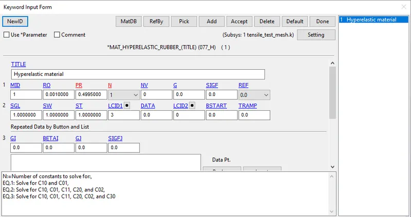
                                                                     Defining MAT_077_H material model

• The simulation has to be repeated for higher order polynomials to check which one fits better to the given input data. So, the simulation is repeated for N=2 and 3 curve fitting cases.

• In the second case, material is modelled using *MAT_OGDEN_RUBBER (077_O) model.
• Parameters such as density, Poisson's ratio, number of constants to solve for (N) are input in the material card.
• Similar to the previous case, initially the curve is fitted with a ploynomial of order 1, i.e., N is set to 1.
• The defined Eng. Stress-Strain curve is given as input for the Strain Energy-Stretch curve fitting, through LCID1 parameter.

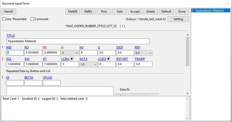
                                                                     Defining MAT_077_O material model

• As in the previous case, the simulation is repeated for N=2 and 3 curve fitting cases.
• The modelled material card and section is assigned to the Dog-Bone specimen in *PART keyword.

 

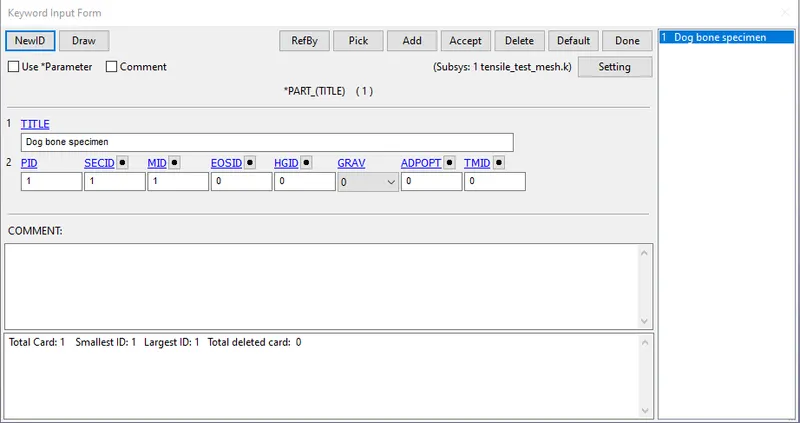
                                                                                        *PART keyword

• Next, the specimen has to be constrained by giving proper boundary conditions.
• One end of the specimen has to be constrained similar to how it is held in the chuck of the UTM.
• The centre nodes on the fixed end of the specimen are constrained in translation and rotation in and about every axis as shown below.

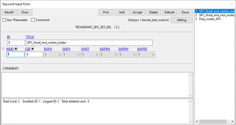
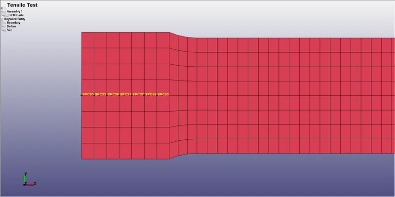
                                                                                              SPC on the centre nodes of fixed end

• Remaining nodes on the fixed end are constrained in translation and rotation in and about every axis except translation in Y-direction as the specimen compression along Y-direction due to Poisson effect.

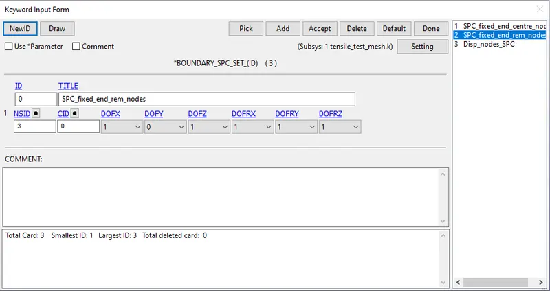
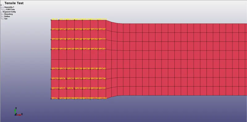
                                                                                          SPC on the remaining nodes of fixed end

• All the nodes on the moving end  are constrained in translation and rotation in and about every axis except translation in X-direction.

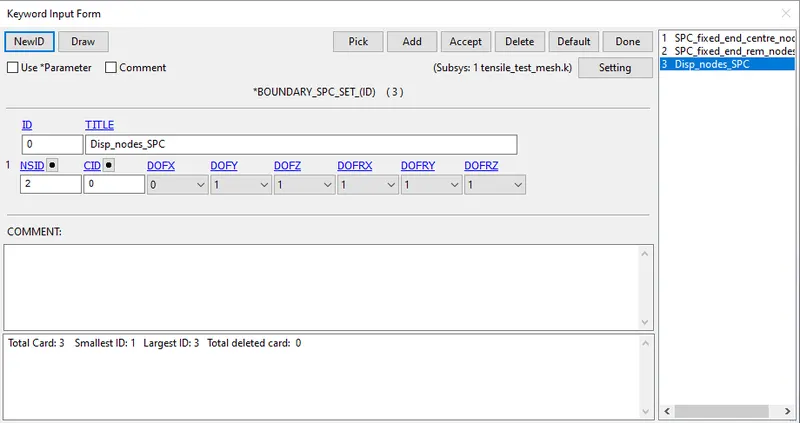
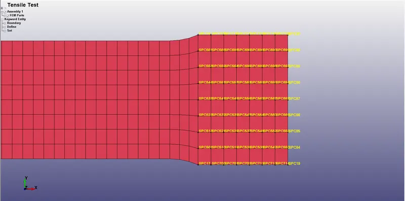
                                                                                                      SPC on the nodes of moving end

• Displacement boundary condition is given to the nodes on the moving end using *BOUNDARY_PRESCRIBED_MOTION_SET keyword as shown below.

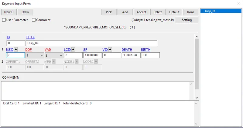
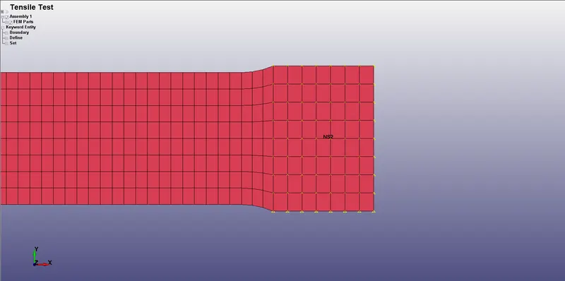
                                                                                   Prescribed motion BC on the nodes of moving end

• Displacement is applied at a constant rate and a displacement of 111 mm (guage length of the specimen) is given to the specimen. The load curve is shown below.

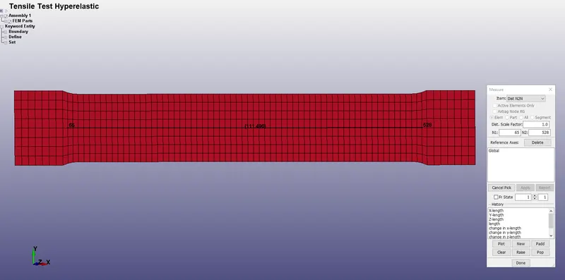
                                                                                            Fig. showing guage length measurement

• Displacement equal to guage length (111 mm) is applied to load the specimen upto a stretch ratio of 2.

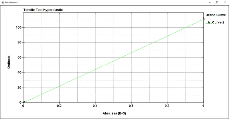
                                                                 Load curve defining the displacement BC

• The tensile test is conducted at a low strain rate without allowing the system to experience any inertial effects. So, the tensile test is actually a static non-linear (material and geometric non-linearity) problem physically.
• Therefore, Implicit solver should be used to solve this problem.
• Implicit method is activated by using *CONTROL_IMPLICIT_GENERAL keyword. The IMFLAG parameter is switched to 1 to activate the implicit method.
• The initial timestep is set to 100 ms. All other options are set to default.

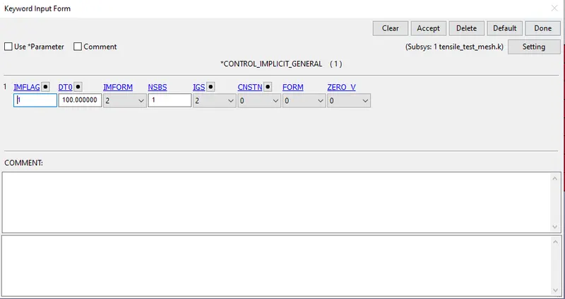
                                                             *CONTROL_IMPLICIT_GENERAL keyword

• Another keyword *CONTROL_IMPLICIT_AUTO is used which controls the time step size for the problem. No. of Equilibrium iterations is set to 11 and iteration window is set to 5 which is the default.

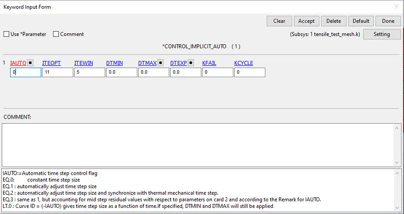
                                                                *CONTROL_IMPLICIT_AUTO keyword

• *CONTROL_IMPLICIT_SOLUTION is defined to activate Non-linear solution method by setting the NSOLVR parameter to 12 as the problem is highly non-linear.

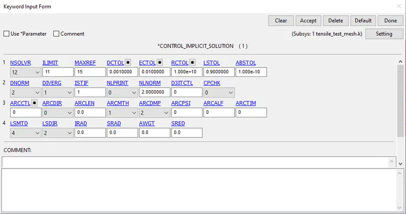
                                                      *CONTROL_IMPLICIT_SOLUTION keyword

• The termination time for the simulation is set to 1000 ms in the *CONTROL_TERMINATION card as shown below.

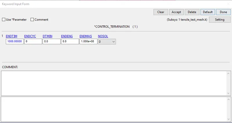
                                                                   *CONTROL_TERMINATION keyword

• At last, the required outputs should be requested using *DATABASE card.
  
  • *DATABASE_BINARY_D3PLOT - Animation file is requested using this card.
  • *DATABASE_EXTENT_BINARY - Strain data are written to the animation d3plot file using this card.

RESULTS AND DISCUSSIONS :

Case I - *MAT_HYPERELASTIC_RUBBER (077_H) model

X-Stress contour plot

• The figure below shows the X-Stress contour when the specimen is in tension.

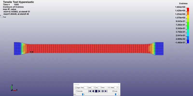
                                                                                                       X-Stress contour plot

• We can observe a max. X-stress of 1.604 MPa at element number 46.

X-Strain contour plot

• The figure below shows the Effective Plastic Strain contour when the specimen is in tension.

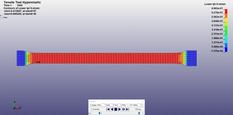
                                                                                                       X-Strain contour plot

• We observe a max. X-Strain of 0.6993 at element number 46.

• The first order N=1 fitted material curve data from the input experimental stress-strain data is taken from the d3hsp file which is shown below.

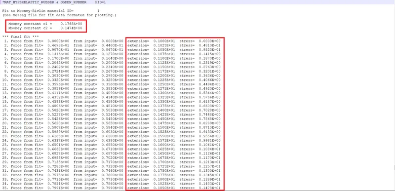
                                                                                  Fitted data in d3hsp file

• The fitted data is in the form of True stress-Stretch ratio data which is highlighted above.
• This True stress-Stretch ratio data is converted into Eng. stress-Eng. strain data using the equations discussed in the introduction.
• This fitted data is plotted in Excel.
• Similarly, the fitted data is taken for N=2 and 3 (2nd and 3rd order polynomial) cases, converted into Eng. stress-Eng. strain data and plotted in Excel.
• N=1,2,3 fitted curves are compared with the input experimental data and the best fit is chosen for material modelling.

  

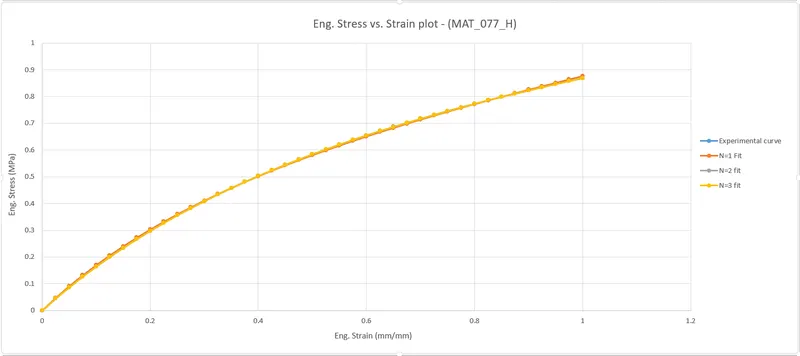
                                                                                     Fit comparison plot

• From the above plot, N=2 and 3 fit curves exactly fit to the input experimental curve.
• N=2 and 3 fit curves provide a perfect fit to the input data. So, the material can be modelled perfectly and efficiently using N=2 fit data.
• The values of constants solved for in N=1 (Mooney-Rivlin), 2 and 3 fit curves are given below.

 

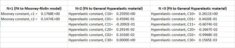
                                                     Constants used to fit the curve in N=1,2 and 3 fit

Case II - *MAT_OGDEN_RUBBER (077_O) model

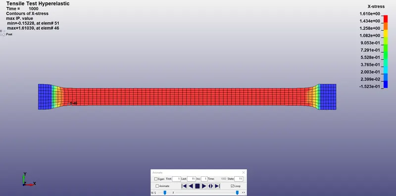
X-Stress contour plot

• The figure below shows the X-Stress contour when the specimen is in tension.

                                                                                                       X-Stress contour plot

• We can observe a max. X-stress of 1.610 MPa at element number 46.

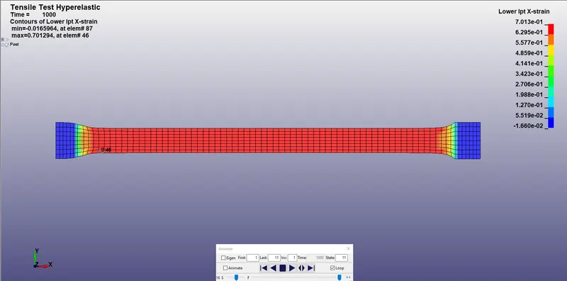
X-Strain contour plot

• The figure below shows the Effective Plastic Strain contour when the specimen is in tension.

                                                                                                       X-Strain contour plot

• We observe a max. X-Strain of 0.7013 at element number 46.

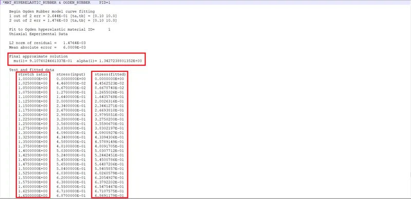
• The first order N=1 fitted material curve data from the input experimental stress-strain data is taken from the d3hsp file which is shown below.

                                                                              Fitted data in d3hsp file

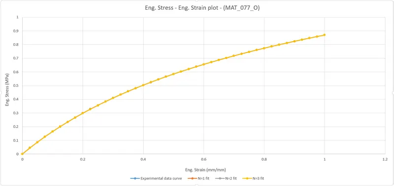
• Similarly, the fitted data is taken for N=2 and 3 (2nd and 3rd order polynomial) cases and plotted in Excel.
• The main difference in this case is that the fitted data is in Eng. stress-Stretch ratio data format. So, only stretch ratio needs to be converted to Eng. strain.

                                                                                        Fit comparison plot

• From the above plot, we can see that N=1,2 and 3 fit curves provide perfect fit to the input data. So, the material can be modelled perfectly and efficiently using N=1 fit data since first order polynomial function reduces the number of constants to be solved for, thereby increasing computational efficiency without any compromise in modelling accuracy.
• The values of constants solved for in N=1, 2 and 3 fit curves are given below.

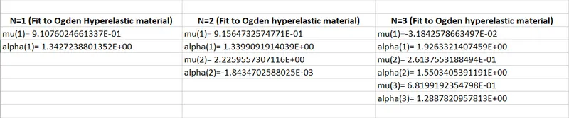
                                                         Constants used to fit the curve in N=1,2 and 3 fit

Material model verification

Case I - *MAT_HYPERELASTIC_RUBBER (077_H) model

• To verify the material model, we should compare the Eng. Stress vs. Eng. Strain plot from the simulation with the same plot which is used to model the material.
• True X-Stress vs. True X-Strain plot from the simulation is extracted from the Element history data by cross-plotting X-stress vs. Time and X-strain vs. Time plots.

 

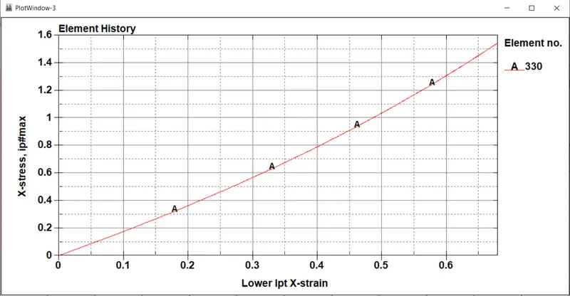
                                                      True X-stress vs. True X-strain plot (by cross-plotting)

• 100 data points are extracted from this plot in .txt file format and this data is imported into MS-Excel.
• The obtained data from the simulation is True stress-strain and the input data used to model the material is Eng. stress-strain data. Therefore, the data is to be converted into Eng. stress-strain data to compare and verify the material model. 
• The converted data is plotted along with the input experimental Eng. Stress-Strain data in Excel to compare and verify how the material behaved in the tensile test simulation.

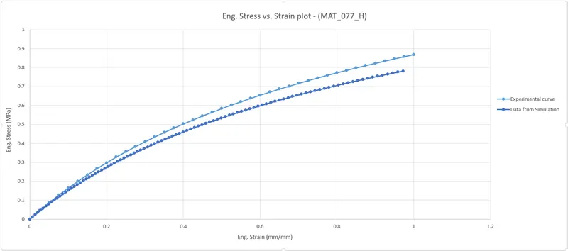
                                                             Verification of the MAT_077_H material model

Case II - *MAT_OGDEN_RUBBER (077_O) model

• In the same manner as in the previous case, the converted Eng. stress-strain data is plotted along with the input experimental Eng. Stress-Strain data in Excel for verification of *MAT_OGDEN_RUBBER (077_O) model.

 

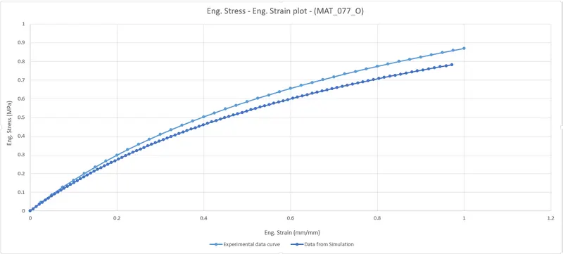
                                                              Verification of the MAT_077_O material model

CONCLUSION :

     From the given material data, *MAT_HYPERELASTIC_RUBBER (077_H) and *MAT_OGDEN_RUBBER (077_O) material cards are modelled and for each material model, the best polynomial fit for Strain energy-Stretch ratio curve is found out. For both the material models, N=3 gave the best fit curve. But, taking computational efficiency in account, *MAT_HYPERELASTIC_RUBBER (077_H) material card can be modelled using N=2 fit data and *MAT_OGDEN_RUBBER (077_O) material card can be modelled using N=1 fit data since they also provide a reasonable fitted curve for the given Eng. Stress-Strain data.