Week - 8 Mass Scaling

AIM :

        To use mass scaling to reduce the runtime of the analysis and ensure the stability of mass scaling.

TOOLS REQUIRED :

• LS-PrePost
• LS-Run

PROCEDURE :

• The given model is opened in LS-PrePost using File -> Open -> LS-DYNA Keyword File option.

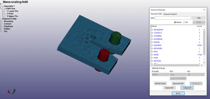
• The deck for the simulation is already completely prepared in the input file.
• First, the model is given to LS-DYNA solver without any control in the timestep in explicit mode.
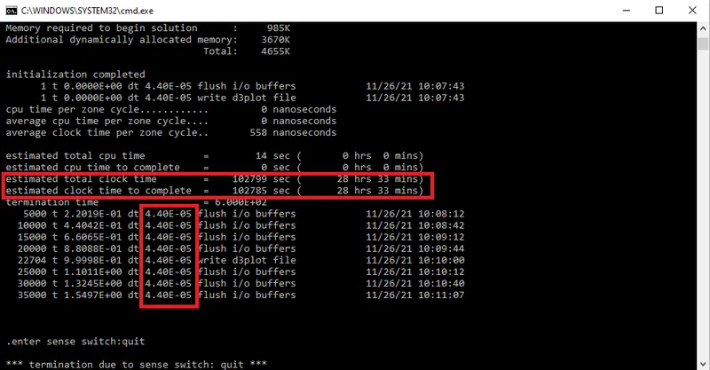
• The solver by itself took a timestep of 4.4E-05 s and showed an estimated run time of 28 hrs 33 mins. The solver window is shown below.

 

• We need to decrease the run time of the simulation by using Mass scaling method.
• In Mass scaling method, the timestep for solving can be increased by adding mass to the components. Mass will be added automatically by the solver.
• Mass should be added only upto a maximum of 8% of the physical mass of the components. Otherwise, the results will deviate very much from the desired range.

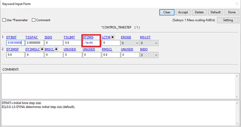
• Mass scaling is enabled by defining *CONTROL_TIMESTEP keyword and minimum timestep size for mass scaled solution is set in the DT2MS parameter.
• In the first trial, DT2MS is set to 1E-04 with a scale factor TSSFAC of 0.9.

• The file is sent to solver and the solver window is shown below.

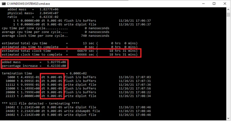
• The timestep got increased to 9E-05 sec from 4.4E-05 sec by adding 1.82E+06 kg mass resulting in 6.4% increase in total mass.
• By increasing the timestep through mass scaling, we could drastically decrease the solver run time to 18 hrs 31 mins. 

• We still have provision to increase the timestep since mass can be added upto 8% of the physical mass.
• In the second trial, DT2MS is increased to 1.1E-04 with a scale factor TSSFAC of 0.9.
• The file is sent to solver and the solver window is shown below.

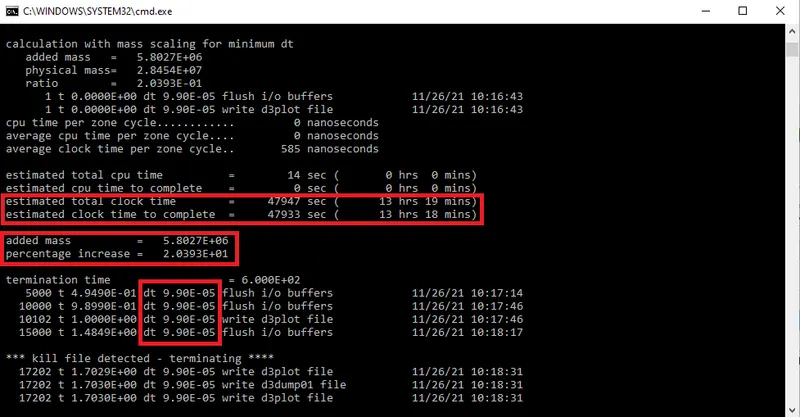
• In the second trial, timestep got increased to 9.9E-05 sec from 9.0E-05 sec by adding 5.8E+06 kg mass resulting in 20.4% increase in total mass. This is very much above the allowable limit of 8%.
• Though the added mass exceeded the limit, we could decrease the solver run time to 13 hrs 18 mins.

• So, we need to decrease the DT2MS value slightly to keep the added mass under limit.
• In the third trial, DT2MS is decreased to 1.02E-04 with a scale factor TSSFAC of 0.9.

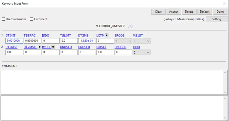
• The file is sent to solver and the solver window is shown below. 

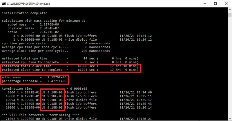
• In the third trial, timestep got decreased to 9.18E-05 sec from 9.9E-05 sec by adding 2.12E+06 kg mass resulting in 7.47% increase in total mass which is under limit.
• The estimated solver run time increased from 13 hrs 18 mins to 17 hrs 10 mins since we decreased the min. allowable timestep for mass scaled solution.

• In the fourth trial, effect of TSSFAC parameter is studied by decreasing the value of TSSFAC and noting the difference in simulation.

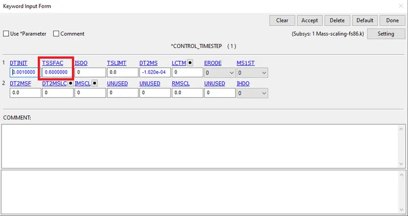
• Here, TSSFAC is set to a min. value 0.6 and submitted to the solver.

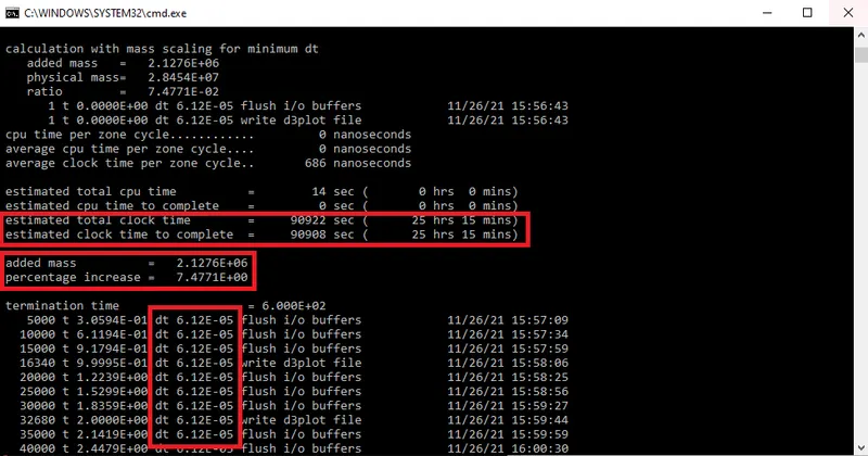
• We can see that the timestep got decreased from 9.18E-05 sec to 6.12E-05 due to the effect of TSSFAC.
• TSSFAC is a scale factor which ensures the stability of the solution by scaling down DT2MS by a factor.
• TSSFAC doesn't have any effect on mass scaling as seen from the solver output shown above. The percentage increase in mass remains same as in the previous case. Mass scaling is controlled by DT2MS only. TSSFAC just makes the solution more stable by scaling down DT2MS.
• A lower TSSFAC actually slows down the solving process by taking lower timesteps to solve the problem. Thus, The solver run time will increase. In this case, the solver run time increased to 25 hrs 15 mins from 17 hrs 10 mins in the case with TSSFAC 0.9.

• So, by enabling the mass scaling option, we could reduce the solver run time by 39% within the 8% limit on mass addition.

Solving by Implicit Method

• The same problem is solved in implicit mode to decide which mode suites better for the problem.
• *CONTROL_IMPLICIT_GENERAL keyword and *CONTROL_IMPLICIT_AUTO keyword are defined to solve the model in implicit mode.

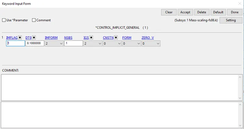
                                                           *CONTROL_IMPLICIT_GENERAL keyword definition

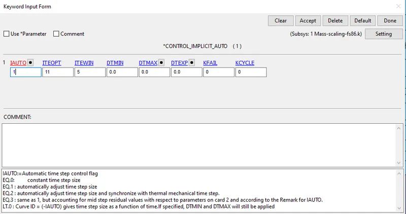
                                                          *CONTROL_IMPLICIT_AUTO keyword definition

• The initial timestep is set to 0.1 in DT0 parameter. All other parameters are set to default.
• The file is sent to solver and the solver window is shown below.

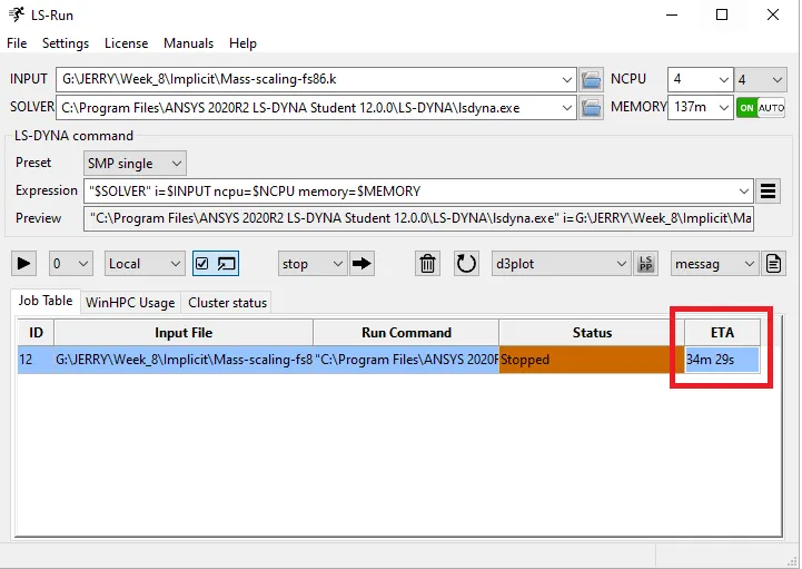
• The solver estimated an approximate run time of 34 mins to solve the problem with default parameters.
• This high run time is due to DT0 parameter which puts a limit on DTMAX (Maximum allowable time step size). By default, DTMAX = DT0*10. This puts a limit on the timestep to not increase beyond 1 in this case.

• So, we increased the DT0 parameter to 10 to see the effect this parameter can make.

 

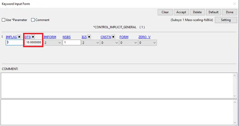
• The file is sent to solver and the solver window is shown below.

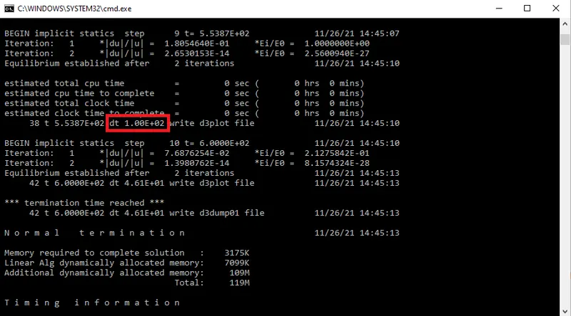
• The solver started with the given DT0 and automatically adjusted to reach a maximum of 100 which is the limit for the given initial timestep.

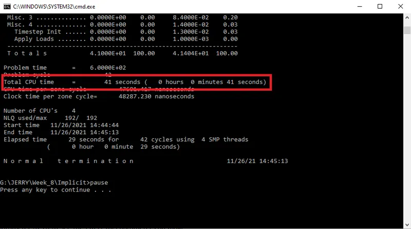
• Just by changing the initial timestep parameter, the run time got drastically reduced from 34 mins to just 41 seconds as shown above.

• In the next trial, the effect of DTMAX is studied by manually controlling the maximum allowable timestep.

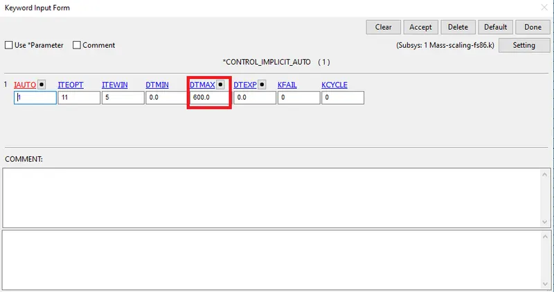
• DTMAX is set to a large value to make the simulation free from the maximum timestep limit constraint as shown in the figure above.
• The file is sent to solver and the solver window is shown below.

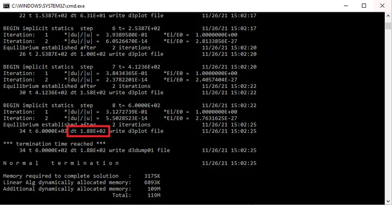
• Now, the limit constraint on maximum timestep is removed and the timestep reached a maximum of 188 without changing the initial timestep DT0.

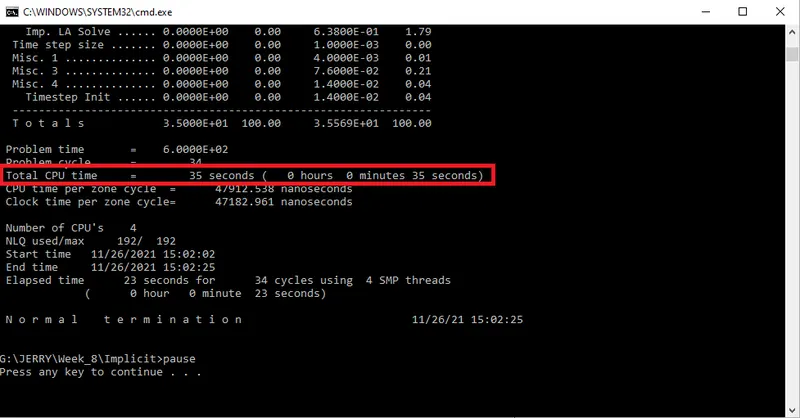
• In this case, we could see a marginal decrease in the run time due to increase in the timestep towards the end of solving. The observed run time is 35 seconds.

• So, by manipulating different parameters in *CONTROL_IMPLICIT_GENERAL keyword and *CONTROL_IMPLICIT_AUTO keyword, we reduced the solver run time by 98%.

RESULT :

• Histogram showing the effect of DT2MS and TSSFAC on Estimated run time is shown below.

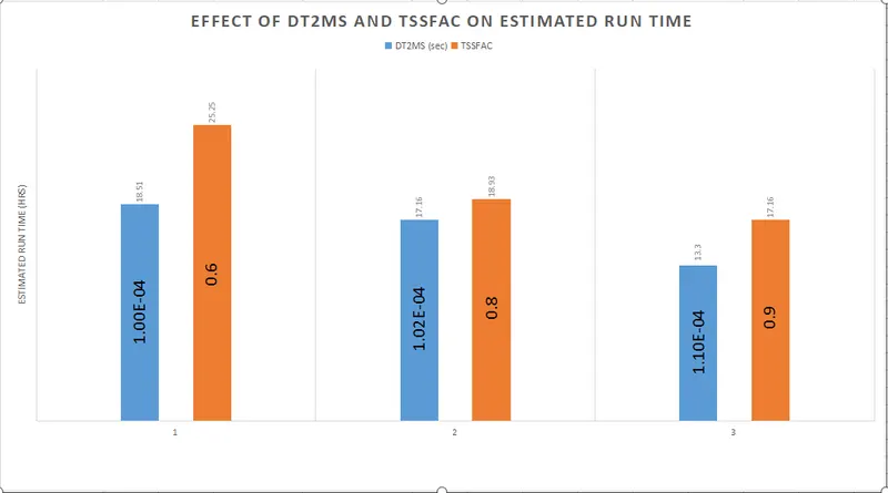
• As DT2MS is increased, the problem will be solved quickly and the run time decreases, provided TSSFAC is kept constant.
• As TSSFAC is increased, the problem will be solved quickly and the run time decreases, provided DT2MS is kept constant.

• Histogram showing the effect of DT2MS and TSSFAC on % increase in mass is shown below.

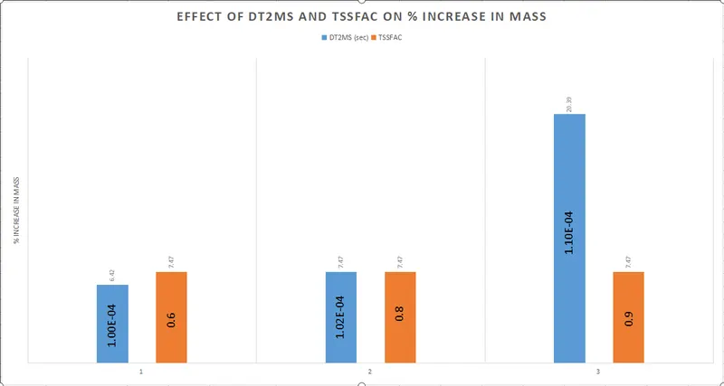
• As DT2MS is increased, more mass addition takes place to satisfy the CFL condition for stability in explicit method.
• TSSFAC does not have any effect on mass addition because TSSFAC scales down the DT2MS to ensure stability. No mass is added for scaling down the timestep.

CONCLUSION :

       The given problem is solved using Explicit and Implicit method and the effect of DT2MS and TSSFAC on mass scaling is studied by trial and error method as discussed above.

• The problem showcases a static event as is clear from the trial and error cases when the problem is aproached through implicit mode.
• The boundary conditions does not impart any dynamic effects throughout the termination time.
• Therefore, the problem can be solved effectively and efficiently by implicit method as the numbers (estimated run time) show.