week-11 Joint creation and Demonstration

AIM :

To demonstrate spherical, revolute, cylindrical, and translational joints between two rigid bodies and two deformable bodies.

TOOLS REQUIRED :

• LS-PrePost
• LS-Run

PROCEDURE :

Mechanical joint is a mechanism which is used to connect one or more mechanical parts to another. The above-mentioned joints will be discussed in the following section.

Spherical Joint

The spherical joint also called a ball joint is shown in figure below. The nodal points 1 and 2 should coincide in the initial configuration. It allows a limited range of smooth movement in all the directions.

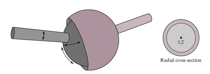
Spherical Joint

Spherical joint between Rigid bodies

• A Ball and Socket FE model is created using Sphere Shell in Shape Mesher in Element and Mesh utility as shown below.

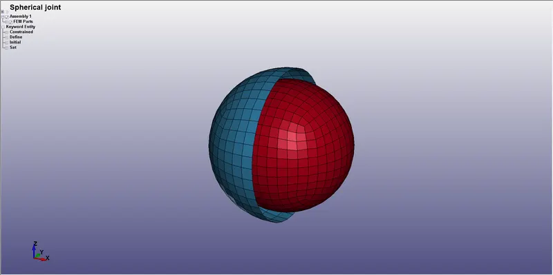
Ball and Socket FE model

• Two additional nodes 10001 and 10002 are created at the same at the centre of the Ball and Socket. These nodes are used for modelling the joint.

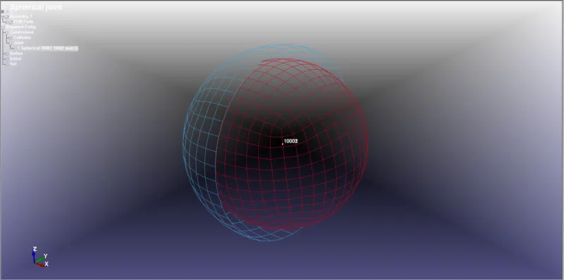
Nodes created for defining joint

• The relative motion of the rigid bodies is constrained so that nodes which are initially coincident remain coincident. In the above figure, the socket’s node is not interior to the socket—LS-DYNA does not require that a rigid body’s nodes be interior to the body.
• The nodes 10001 and 10002 should be added to the Ball and Socket respectively using *CONSTRAINED_EXTRA_NODES_SET keyword as shown below.

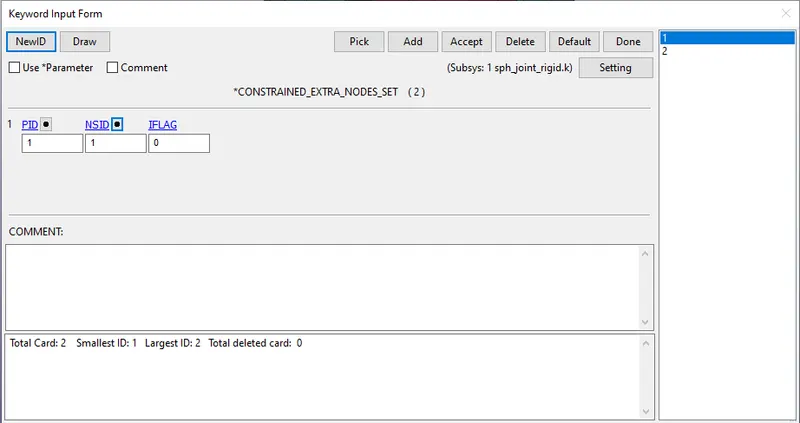
Defining extra nodes to the rigid bodies

• *MAT_RIGID material keyword is assigned for defining rigid material properties for both the parts.
• The socket should be constrained in translation and rotation in and about every axis in the workspace. Since, the part is modelled using rigid material, it is possible to constrain the part in the material card itself using CMO parameter.

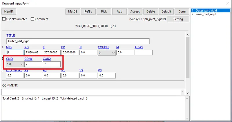
Defining material card

• The ball is assigned with the same *MAT_RIGID card but without the centre of mass constraint option since the ball is to rotate inside the socket.
• The section properties for the model are defined by using *SECTION_SHELL keyword. All the properties are set to default and a thickness of 1mm is assigned to the shell elements.

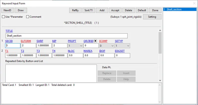
Section definition for the Ball and Socket part

• The joint is defined using *CONSTRAINED_JOINT_SPHERICAL keyword with node 10001 as N1 and 10002 as N2 as shown below.

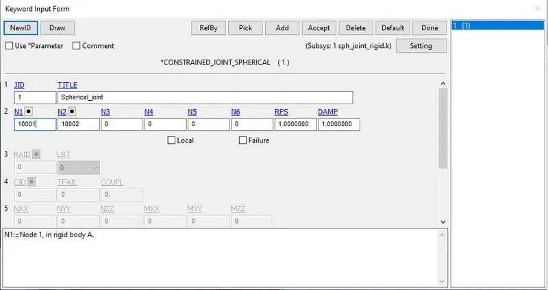
Definition of Spherical joint

• Initial velocity boundary condition is defined to the ball part using *INITIAL_VELOCITY_RIGID_BODY keyword.

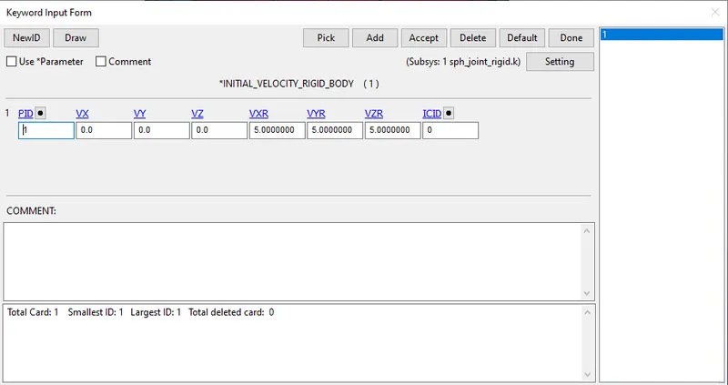
Definition of initial velocity boindary condition

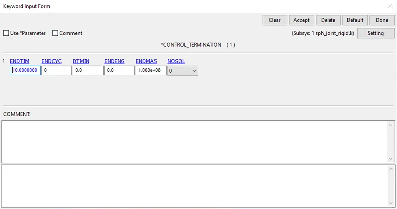
• The termination time for the simulation is set to 10 ms in the *CONTROL_TERMINATION card as shown below.

• *CONTROL_TIMESTEP keyword is added to limit the timestep from going very high to ensure stability of the model.
• The maximum allowed timestep of 0.01 ms is input as a curve through LCTM parameter.

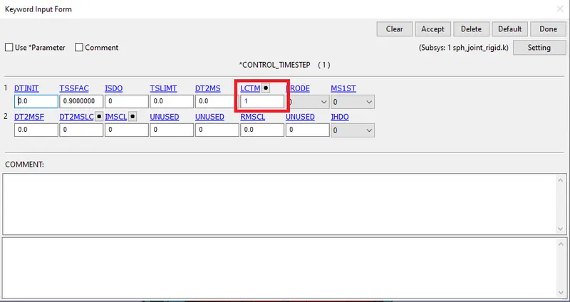
*CONTROL_TIMESTEP keyword

• At last, the required outputs should be requested using *DATABASE card.
  
  • *DATABASE_BINARY_D3PLOT - Animation file is requested using this card.
  • *DATABASE_ASCII_option - Outputs such as Global Statics (GLSTAT), Part Energies (MATSUM).

Spherical joint between Deformable bodies

• In this case, both the ball and socket parts are modelled with a deformable material card *MAT_ELASTIC keyword since the parts to be connected with the joint are deformable.

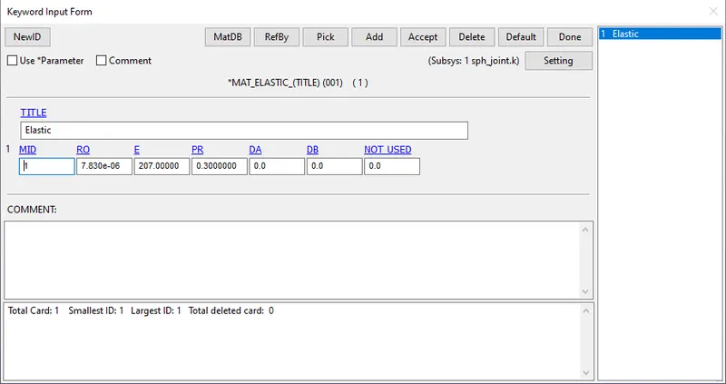
Defining material card

• The section properties for the model are defined by using *SECTION_SHELL keyword. Fully integrated element formulation (ELFORM 16) is used since hourglass effect is observed with default element formulation (ELFORM 2) and a thickness of 1mm is assigned to the shell elements.

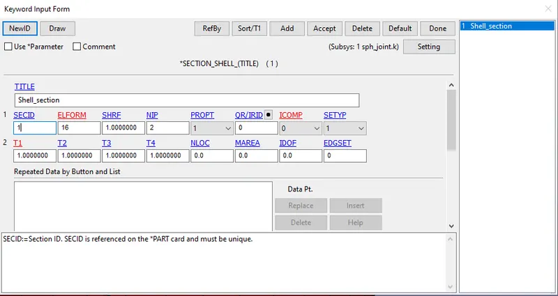
Section definition for the Ball and Socket part

• The nodes 10001 and 10002 should be attached to the Ball and Socket respectively using *CONSTRAINED_NODAL_RIGID_BODY keyword since the parts to be joined are deformable as shown below.

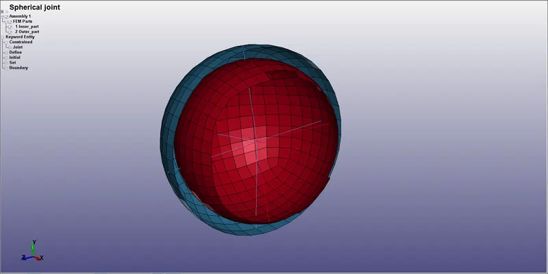
CNRB definition

• The joint is defined using *CONSTRAINED_JOINT_SPHERICAL keyword with node 10001 as N1 and 10002 as N2 in the same manner as in the rigid body case.
• Next, the socket is constrained in workspace using *BOUNDARY_SPC_SET keyword. The nodes added to CNRB is excluded from this SPC since it will over-constrain the nodes.

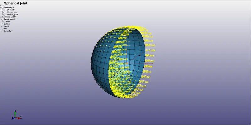
SPC definition for Socket

• Initial velocity boundary condition is defined to the ball part using *INITIAL_VELOCITY_GENERATION keyword with the part ID and angular velocity as input.
• The axis about which rotation is to be given is defined by giving corresponding direction cosines (NX, NY, NZ).

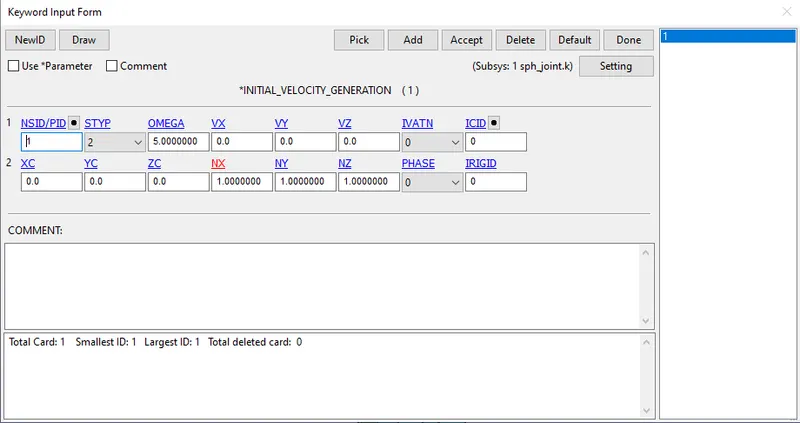
Definition of initial velocity boundary condition

• The remaining keywords are defined exactly similar to the previous case.
• The model is submitted to the solver.

Revolute Joint

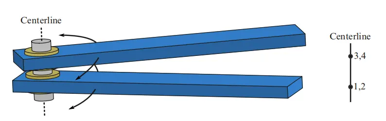
Revolute joint

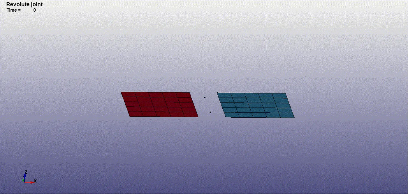
Nodes 1 and 2 are coincident; nodes 3 and 4 are coincident. Nodes 1 and 3 belong to rigid body A; nodes 2 and 4 belong to rigid body B. The relative motion of the two rigid bodies is restricted to rotations about the axis formed by the two pairs of coincident nodes. This axis is labeled the “centerline.”

Revolute joint between Rigid bodies

• Two simple shell plate FE model is created using 4N Shell in Shape Mesher in Element and Mesh utility as shown below.

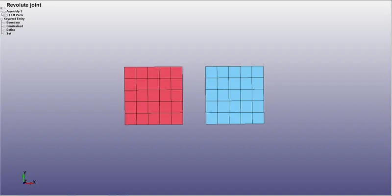
Plate shell parts

• Four additional nodes 501, 502, 503 and 504 are created to define the axis of the revolute joint as shown below. These nodes are used for modelling the joint.

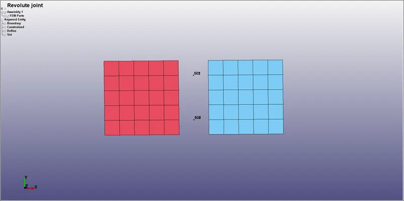
Nodes created for defining joint

• Node pairs (501,502) and (503,504) should be coincident in this case to define the revolute joint.
• The nodes 501 and 503 should be added to Part 1 (Red) and nodes 502 and 504 should be added to Part 2 (Blue) using *CONSTRAINED_EXTRA_NODES_SET keyword as shown below.
• Material and section are defined similar to the corresponding case in spherical joint.

• The joint is defined using *CONSTRAINED_JOINT_REVOLUTE keyword with node 501 as N1, 502 as N2, 503 as N3 and 504 as N4 as shown below.

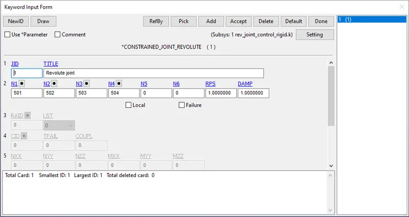
Definition of Revolute joint

• Prescribed motion boundary condition is defined to Part 2 (Blue) using *BOUNDARY_PRESCRIBED_MOTION_NODE keyword.
• One of the outer edge nodes is given displacement boundary condition in the global Z-direction, input using a curve.

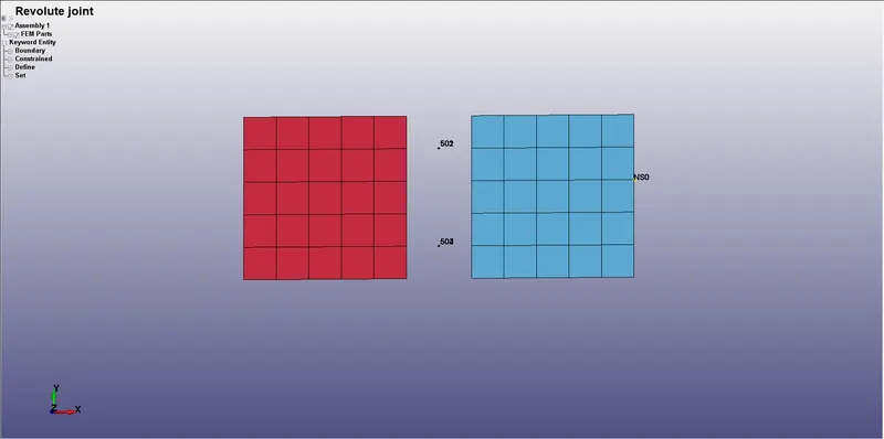
Prescribed motion boundary condition

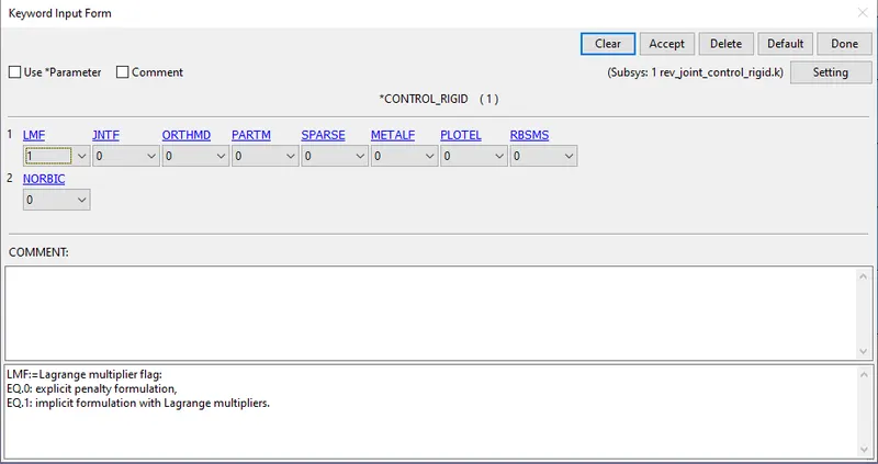
• *CONTROL_RIGID keyword is also defined to increase the joint stiffness to ensure the stability of the joint.
• In *CONTROL_RIGID keyword, Lagrange multiplier flag (LMF) is set to 1, i.e., implicit formulation with Lagrange multipliers.

• All the remaining keyword cards are defined similar to the corresponding case in the spherical joint.
• The model is submitted to the solver.

Revolute joint between Deformable bodies

• In this case, both the parts are modelled with a deformable material card *MAT_ELASTIC keyword since the parts to be connected with the joint are deformable.
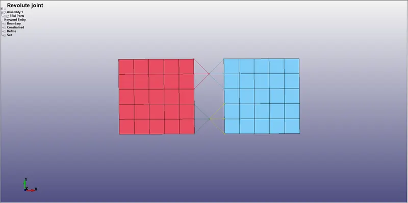
• The nodes 501 and 503 should be attached to Part 1 and nodes 502 and 504 should be attached to Part 2 using *CONSTRAINED_NODAL_RIGID_BODY keyword since the parts to be joined are deformable as shown below.

CNRB definition

• The joint is defined using *CONSTRAINED_JOINT_REVOLUTE keyword with node 501 as N1, 502 as N2, 503 as N3 and 504 as N4 in the same manner as in the rigid body case.
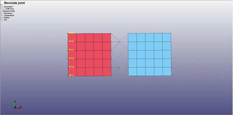
• Next, Part 1 is constrained in workspace using *BOUNDARY_SPC_SET keyword. The nodes added to CNRB is excluded from this SPC since it will over-constrain the nodes.

• Prescribed motion boundary condition is defined to Part 2 (Blue) using *BOUNDARY_PRESCRIBED_MOTION_NODE keyword in the same manner as above.
• The remaining keywords are defined exactly similar to the previous case.
• The model is submitted to the solver.

Cylindrical joint

Cylindrical joint

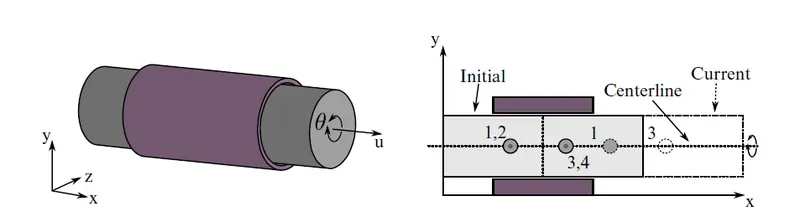
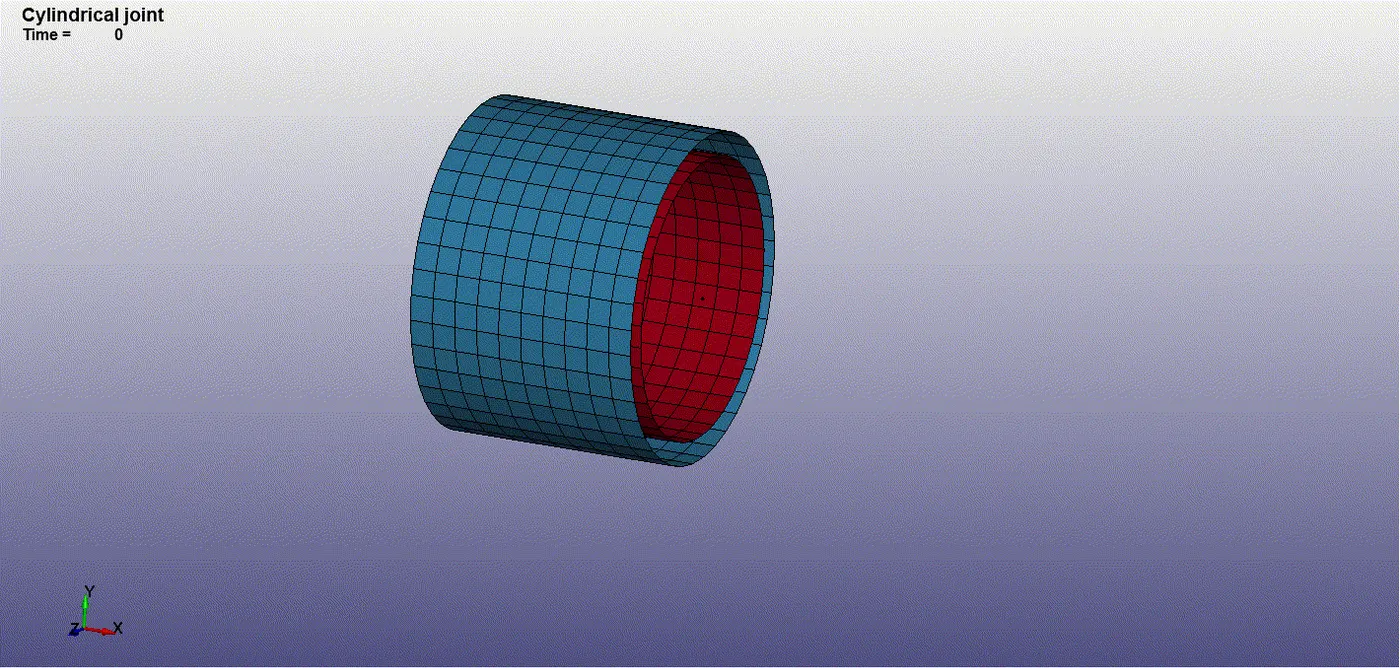
This joint is derived from the rotational joint by relaxing the constraints along the centerline. This joint admits relative rotation and translation along the centerline.

Cylindrical joint between Rigid bodies

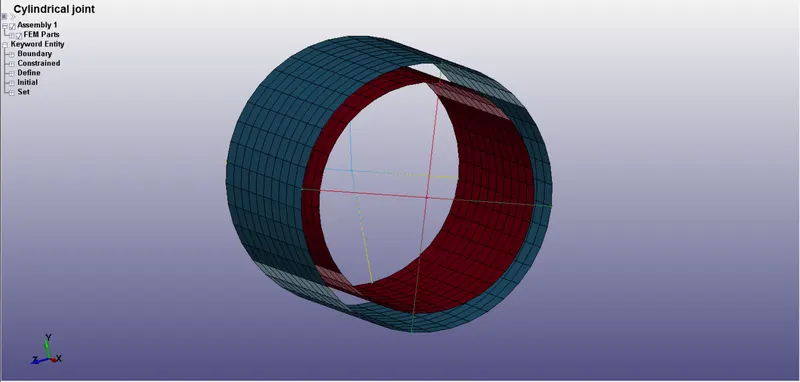
• Two concentric cylindrical shell part FE model is created using Cylinder Shell in Shape Mesher in Element and Mesh utility as shown below.

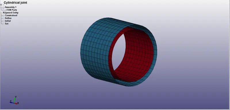
Concentric cylindrical shell parts

• Four additional nodes 1001, 1002, 1003 and 1004 are created to define the axis of the cylindrical joint as shown below. These nodes are used for modelling the joint.

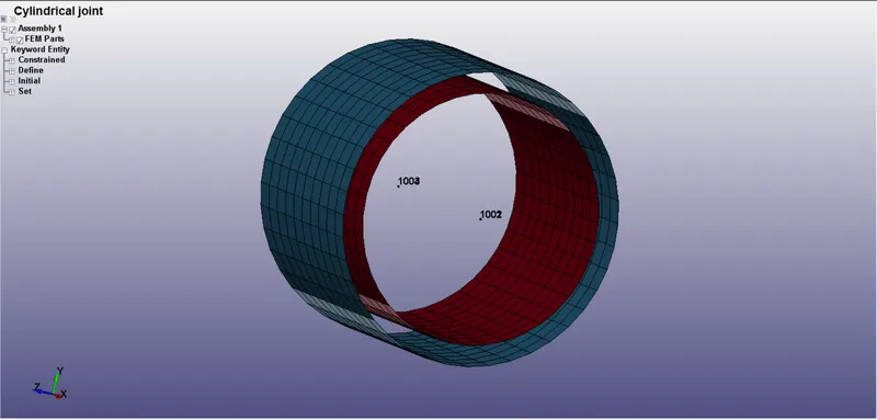
Nodes created for defining joint

• Node pairs (1001,1002) and (1003,1004) should be coincident in this case to define the cylindrical joint.
• The nodes 1001 and 1003 should be added to Part 1 (Red) and nodes 1002 and 1004 should be added to Part 2 (Blue) using *CONSTRAINED_EXTRA_NODES_SET keyword.
• Material and section are defined similar to the corresponding case in revolute joint.

• The joint is defined using *CONSTRAINED_JOINT_CYLINDRICAL keyword with node 1001 as N1, 1002 as N2, 1003 as N3 and 1004 as N4 as shown below.

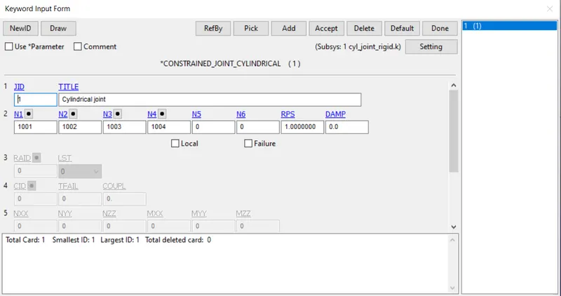
Definition of Cylindrical joint

• Initial velocity boundary condition is defined to Part 1 using *INITIAL_VELOCITY_RIGID_BODY keyword.

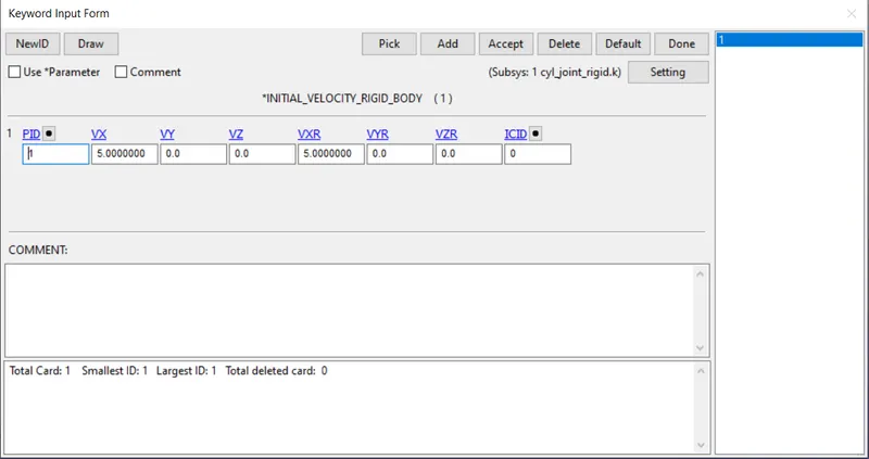
Definition of initial velocity boundary condition

• All the remaining keyword cards are defined similar to the corresponding case in the spherical joint.
• The model is submitted to the solver.

Cylindrical joint between Deformable bodies

• In this case, both the parts are modelled with a deformable material card *MAT_ELASTIC keyword since the parts to be connected with the joint are deformable.
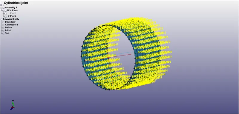
• The nodes 1001 and 1003 should be attached to Part 1 and nodes 1002 and 1004 should be attached to Part 2 using *CONSTRAINED_NODAL_RIGID_BODY keyword since the parts to be joined are deformable as shown below.

CNRB definition

• The joint is defined using *CONSTRAINED_JOINT_CYLINDRICAL keyword with node 1001 as N1, 1002 as N2, 1003 as N3 and 1004 as N4 in the same manner as in the rigid body case.
• Next, Part 2 is constrained in workspace using *BOUNDARY_SPC_SET keyword. The nodes added to CNRB is excluded from this SPC since it will over-constrain the nodes.

• Initial velocity boundary condition is defined to the Part 1 using *INITIAL_VELOCITY_GENERATION keyword with the part ID and angular velocity as input.
• The axis about which rotation is to be given is defined by giving corresponding direction cosines (NX, NY, NZ).

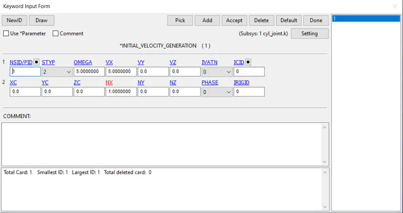
Definition of initial velocity boundary condition

• The remaining keywords are defined exactly similar to the previous case.
• The model is submitted to the solver.

Translational joint

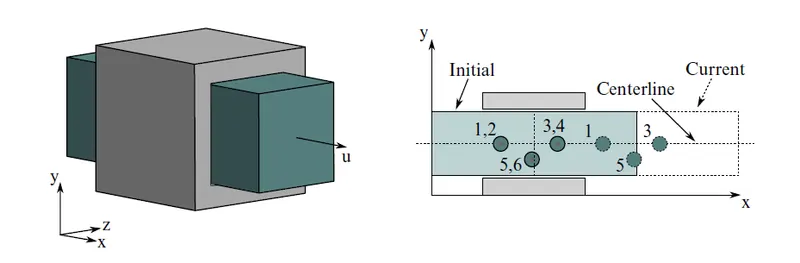
Translational joint

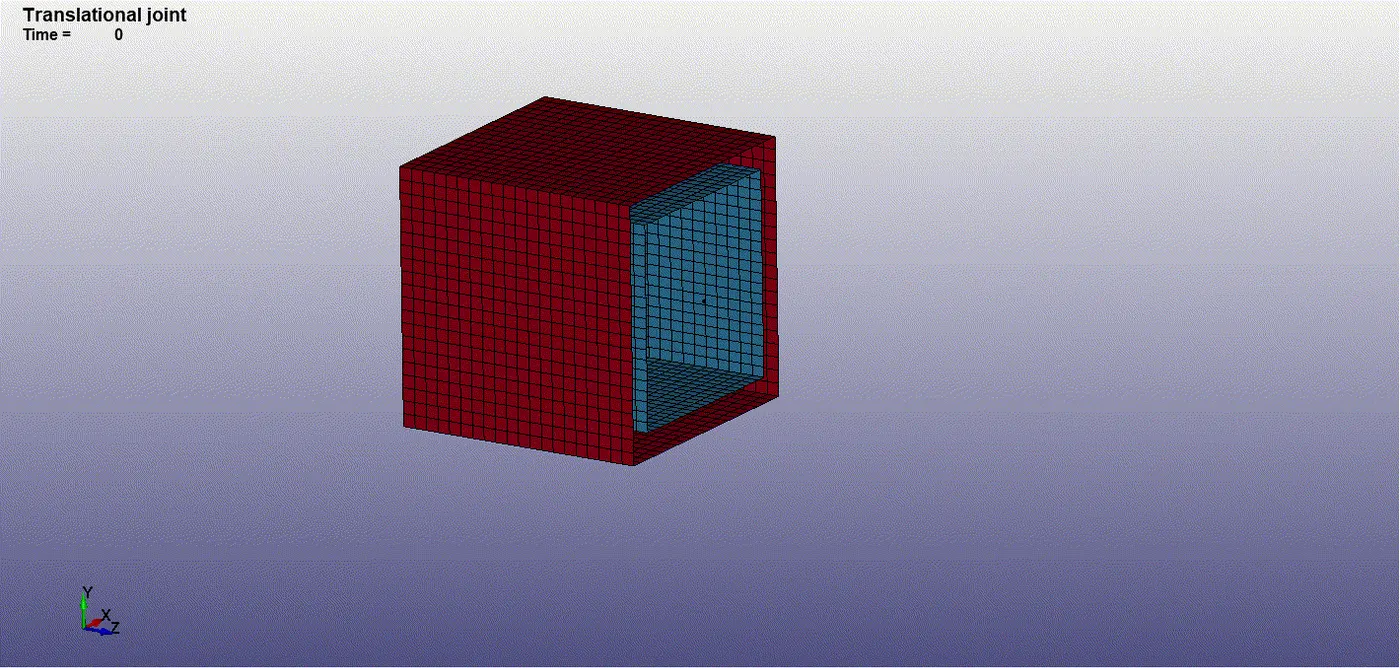
This is a cylindrical joint with a third pair of off-centerline nodes which restrict rotation. Aside from translation along the centerline, the two rigid bodies are stuck together.

Cylindrical joint between Rigid bodies

• Two concentric cubic shell part FE model is created using Box Shell in Shape Mesher in Element and Mesh utility as shown below.

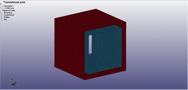
Concentric cubic shell parts

• Six additional nodes 10001, 10002, 10003, 10004, 10005 and 10006 are created to define the axis of the translational joint as well as to constrain the rotation about the joint axis as shown below. These nodes are used for modelling the joint.

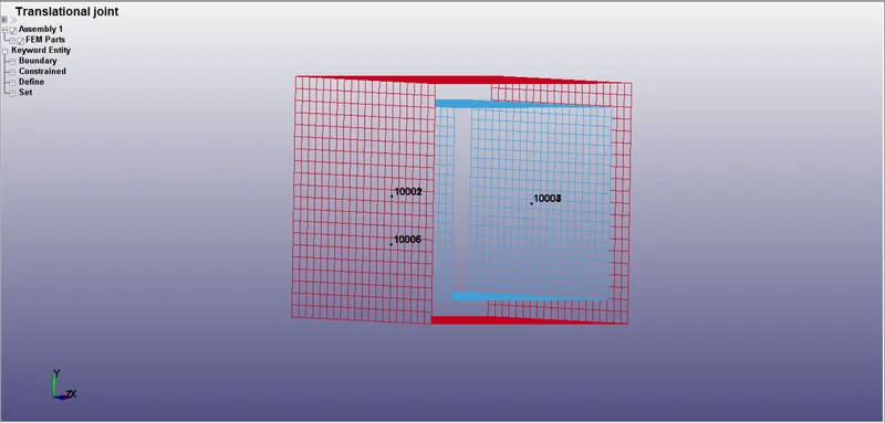
Nodes created for defining joint

• Node pairs (10001,10002), (10003,10004) and (10005,10006) should be coincident in this case to define the translational joint.
• The nodes 10001, 10003 and 10005 should be added to Part 2 (Blue) and nodes 10002, 10004 and 10006 should be added to Part 1 (Red) using *CONSTRAINED_EXTRA_NODES_SET keyword.
• Material and section are defined similar to the corresponding case in translational joint.

• The joint is defined using *CONSTRAINED_JOINT_TRANSLATIONAL keyword with node 10001 as N1, 10002 as N2, 10003 as N3, 10004 as N4, 10005 as N5 and 10006 as N6 as shown below.

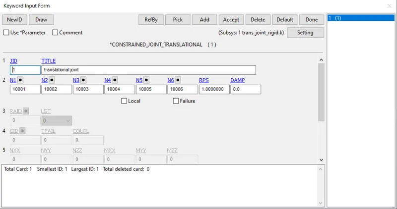
Definition of Translational joint

• Initial velocity boundary condition is defined to Part 2 using *INITIAL_VELOCITY_RIGID_BODY keyword.

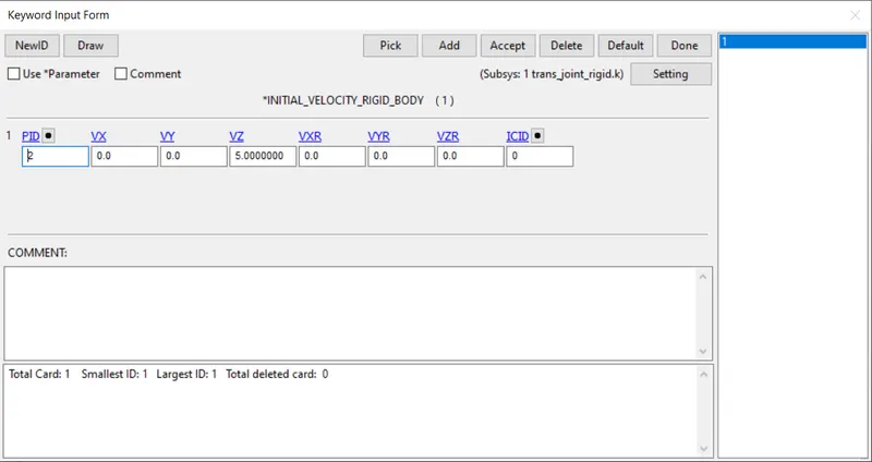
Definition of initial velocity boundary condition

• All the remaining keyword cards are defined similar to the corresponding case in the spherical joint.
• The model is submitted to the solver.

Translational joint between Deformable bodies

• In this case, both the parts are modelled with a deformable material card *MAT_ELASTIC keyword since the parts to be connected with the joint are deformable.
• The nodes 10001, 10003 and 10005 should be attached to Part 2 and nodes 10002, 10004 and 10006 should be attached to Part 1 using *CONSTRAINED_NODAL_RIGID_BODY keyword since the parts to be joined are deformable as shown below.

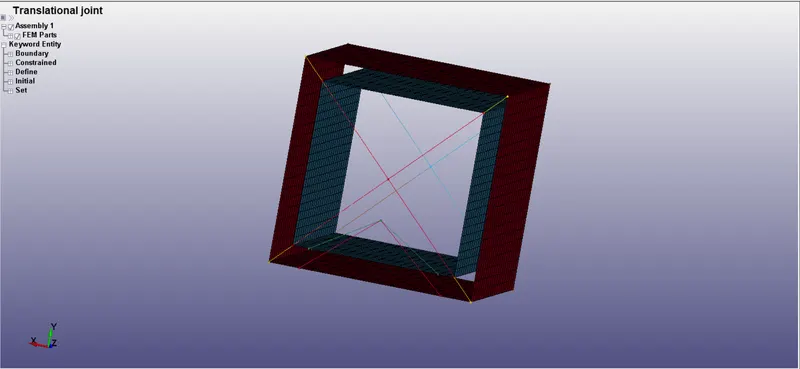
CNRB definition

• The joint is defined using *CONSTRAINED_JOINT_TRANSLATIONAL keyword with node 10001 as N1, 10002 as N2, 10003 as N3, 10004 as N4, 10005 as N5 and 10006 as N6 in the same manner as in the rigid body case.
• Next, Part 1 is constrained in workspace using *BOUNDARY_SPC_SET keyword. The nodes added to CNRB is excluded from this SPC since it will over-constrain the nodes.

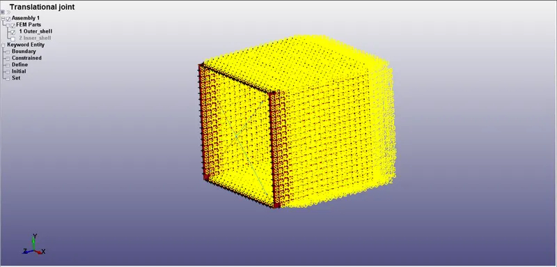
• Initial velocity boundary condition is defined to the Part 2 using *INITIAL_VELOCITY_GENERATION keyword with the part ID and angular velocity as input.
• The axis about which rotation is to be given is defined by giving corresponding direction cosines (NX, NY, NZ).

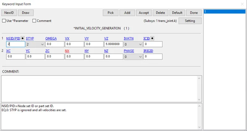
Definition of initial velocity boundary condition

• The remaining keywords are defined exactly similar to the previous case.
• The model is submitted to the solver.

RESULTS :

Animation of Spherical joint

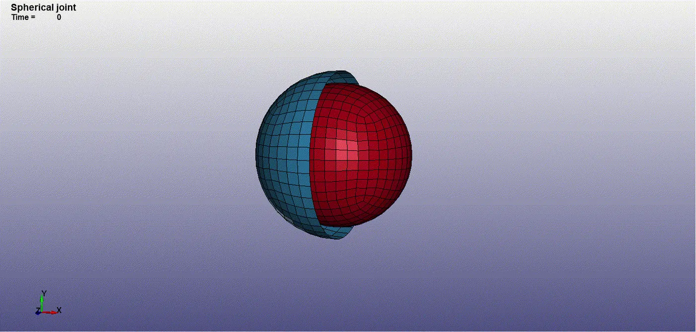
Animation of Revolute joint

Animation of Cylindrical joint

Animation of Translational joint

CONCLUSION :

All the types of joints - Spherical, Revolute, Cylindrical and Translational have been modelled and demonstrated.