Week - 2 - Explicit and Implicit Analysis
AIM :
To solve the below Force-Displacement non-linear response of a material using both explicit and implicit methods and to compare the results to find out which method gives better approximate results.
The Force-Displacement relation is given below :
`f(u) = u^3+9u^2+4u`
where,
u - displacement
f(u) - internal force generated due to the application of external force, which is a function of displacement.
THEORY :
Explicit Method
The explicit method allows solving problems element by element. Compared with the implicit method, it does not require the general matrix, since the velocity and displacement nodes can be counted directly, using the central difference integration scheme. However, the time step is limited by the size of the numerical stability. Accordingly, this method is considered as conditionally stable, because if the time step is too large, there will be a significant numerical error. In this method, there is no requirement for balance, so it is suitable for highly dynamic analysis, such as high velocity impact. Explicit finite element codes are now used extensively in aerospace, nuclear, and rail technology. In this way, bird strike, safety of transport bottles, train crash, etc., can be simulated. The best-known commercial software analyses for the explicit method are: PAM-CRASH, LS-DYNA, and RADIOSS.
Implicit Method
An implicit method requires the formation of a global stiffness matrix [K]. In static problems, the equilibrium is maintained when [K]−1 is multiplied to both sides of the static equilibrium equation. After that, nodal displacements can be easily calculated. One disadvantage of carrying out this operation is that large sizes of storage space and in-core memory are needed to find [K]−1. Additionally, nonlinearity causes [K] to become a function of displacement. As such, updating or factorizing the global stiffness matrix [K] before inverting it to [K]−1 for computing the nodal displacements needed before the next time step can be proceed is computationally intensive.
SOLUTION :
The given Force-Displacement response is given by,
`f(u)=u^3+9u^2+4u`
We know that the stiffness of the material is given by the first derivative of the Force-Displacement relation.
`k(u)=(df)/(du)= 3u^2+18u+4`
Explicit Method
`u_i` - displacement at 'i' th step
`k(u)` - stiffness of the material which is a function of displacement
`DeltaF` - Incemental change in externally applied force
`Deltau_i` - Change in displacement at 'i' th step
`(F_(ext))_i` - Externally applied force at 'i' th step
`f_(i)` - internal force generated at 'i' th step
Step 1
Initial displacement, `u_0` = 0
Initial stiffness, `k(u_0)` = `3*(0)^2+18*0+4` = 4 units
`DeltaF` = 1 unit
`Deltau_1=(DeltaF)/(k(u_0))=1/4=0.25` units
`u_1=u_0+Deltau_1=0+0.25=0.25` units
Step 2
`u_1 =0.25` units
Updated stiffness, `k(u_1)` = `3*(0.25)^2+(18*0.25)+4` = 8.6875 units
`DeltaF` = 1 unit
`Deltau_2=(DeltaF)/(k(u_1))=1/8.6875=0.1151` units
`u_2=u_1+Deltau_2=0.25+0.1151=0.3651` units
Step 3
`u_2 =0.3651` units
Updated stiffness, `k(u_2)=3*(0.3651)^2+(18*0.3651)+4` = 10.971 units
`DeltaF` = 1 unit
`Deltau_3=(DeltaF)/(k(u_2))=1/10.971=0.0911` units
`u_3=u_2+Deltau_3=0.3651+0.0911=0.4562` units
At the end of the third step,
`F_(ext)=3` units
Internal force, `f=(u_3)^3+9(u_3)^2+4u_3=3.79` units
It is evident from the results that external and internal forces are NOT in equilibrium because `F_(ext)!=f`. Table summarizes the main results for the explicit analysis.
| Step,`i` | `DeltaF_i` | `Deltau_i` | `u_i` | `(F_(ext))_i` | `f_i` | `R=f_i-(F_(ext))_i` |
| 1 | 1 |
0.25 |
0.25 | 1 | 1.578 | 0.578 |
| 2 | 1 | 0.1151 | 0.3651 | 2 | 2.708 | 0.708 |
| 3 | 1 | 0.0911 | 0.4562 | 3 | 3.792 | 0.792 |
Implicit Method
`u_i` - displacement at 'i' th step
`k(u)` - stiffness of the material which is a function of displacement
`DeltaF` - Incemental change in externally applied force
`Deltau_i` - Change in displacement at 'i' th step
`(F_(ext))_i` - Externally applied force at 'i' th step
`f_(i)` - internal force generated at 'i' th step
`R(u)` - Residual = `abs(f_i-(F_(ext))_i)`
Tolerance = `10^-2` (user-defined)
`deltau^((j))` - Correction to `u_i` in the 'j' th Newton-Raphson iteration
`u_i^((j))` - displacement at 'i' th step in the 'j' th Newton-Raphson iteration
Step 1
Initial displacement, `u_0` = 0
Initial stiffness, `k(u_0)` = `3*(0)^2+18*0+4` = 4 units
`DeltaF` = 1 unit
`Deltau_1=(DeltaF)/(k(u_0))=1/4=0.25` units
`u_1=u_0+Deltau_1=0+0.25=0.25` units
Checking the residual,
`f_1=(u_1)^3+9(u_1)^2+4u_1=1.578` units
Tolerance = `10^-2`
Residual, `R^((0))=f_1-(F_(ext))_1=1.578-1=0.578`
`R^((0))>10^-2`
Therefore, applying Newton-Raphson iteration 1,
`deltau^((1))=-[k(u_1^((0)))]^-1*R^((0))`
`k(u_1^((0)))=k(0.25)=8.6875` unit`
`deltau^((1))=-(8.6875)^-1*0.578=-0.0665` units
Corrected `u_1=u_1^((1))=u_1^((0))+deltau^((1))=0.25-0.0665=0.1835` units
Checking the residual again,
`f_1=(u_1^((1)))^3+9(u_1^((1)))^2+4u_1^((1))=1.0432` units
`R^((1))=1.0432-1=0.0432`
`R^((1))>10^-2`
Therefore, applying Newton-Raphson iteration 2,
`deltau^((2))=deltau^((1))-[k(u_1^((1)))]^-1*R^((1))`
`k(u_1^((1)))=k(0.1835)=7.404` units
`deltau^((2))=-0.0665-(7.404)^-1*0.0432=-0.0723` units
Corrected `u_1=u_1^((2))=u_1^((0))+deltau^((2))=0.25-0.0723=0.1777` units
Checking the residual again,
`f_1=(u_1^((2)))^3+9(u_1^((2)))^2+4u_1^((2))=1.0006` units
`R^((2))=1.0006-1=0.0006`
`R^((2))<10^-2`
Residual has come inside the tolerance value.
Therefore, no further iterations needed.
Final value of `u_1=u_1^((2))=0.1777` units
Similarly, steps 2 and 3 are carried out and the results are shown in the table below.
| Step `i` | `DeltaF_i` | `u_i` | `(F_(ext))_i` | `f_i` | `R=abs(f_i-(F_(ext))_i)` |
| 1 | 1 | 0.1777 | 1 | 1.0006 | 0.0006 |
| 2 | 1 | 0.2966 | 2 | 2.0042 | 0.0042 |
| 3 | 1 | 0.3911 | 3 | 3.0008 | 0.0008 |
It is evident from the table that the external forces and internal forces are coming into equilibrium.
RESULTS AND OBSERVATIONS :
The following table shows the convergence in explicit and implicit method. We can see that the residual in implicit method in each step is much lower when compared to explicit method. This is because, in implicit method, convergence check is made in each step before proceding to the next step. Therefore, force balance is ensured in each step which is not in case of explicit method. From the residual values, we can clearly infer that the implicit method gives better approximate results in the given problem.
| Steps | Residual (R) in Explicit method | Residual (R) in Implicit method |
| 1 | 0.578 | 0.0006 |
| 2 | 0.708 | 0.0042 |
| 3 | 0.792 | 0.0008 |
The graph showing the comparison of explicit and implicit method is shown below.
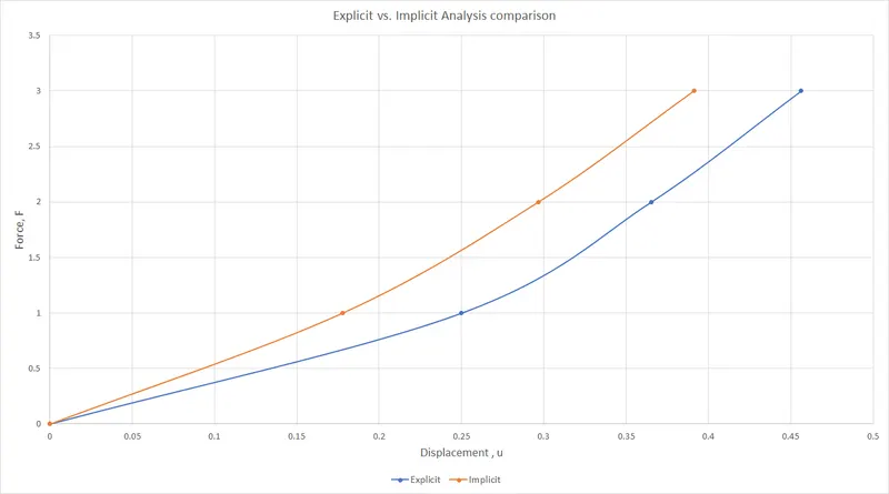
From the table of implicit method, we have seen that the externally applied force `F_(ext)` and internal force `f` are coming into almost an equilibrium in each step based on the tolerance we define. This is not in the case of explicit method where residual is not taken into account. Since equilibrium is attained in each step in case of implicit method, we can say that implicit method results are way more close to the analytical results in the above problem. Therefore, as we can see from the comparison plot, explicit method results deviate very much from the implicit method results which implies that implicit method gave better approximate results than explicit method in the present problem model. This doesn't mean that implicit method always give better results in any type of problem. Solution method have to be decided according to the type of analysis like whether it is linear or non-linear and whether it is static, quasistatic or dynamic. Even explicit method can be used to get a better approximate results by decreasing the load increment step (`DeltaF`) and performing more number of steps.
CONCLUSION :
The given non-linear static problem is solved using both explicit and implicit methods to find out the feasibility of both methods in the particular problem. From the results, we came to the conclusion that implicit method will give better results in non-linear static problems like the given one when different factors like time and computational cost is taken into consideration.