Frontal Crash Analysis of DODGE Neon BIW model using HyperMesh and RADIOSS

AIM :

To conduct the vehicle Frontal Crashworthiness test on the given BIW model of Dodge Neon as per Federal Motor Vehicle Safety Standards (FMVSS) 208 using RADIOSS and analyse the results using HyperView and HyperGraph 2D.

OBJECTIVES :

• Check unit system and either follow[Mg mm s] or [Kg mm ms].
• Create appropriate interface ,friction 0.2 and recommended parameters.
• Make sure of no penetrations and intersection.
• Correct rigid bodies if any issues.
• Create rigid wall with friction 0.1.
• Compare the model weight with the full scale 300k nodes model and use added masses to reach target weight 700kg while getting CG about the required range.
• Initial velocity 35 mph.
• Use model checker to ensure good quality.
• Time-step :0.5 to 0.1 microseconds.
• Run 80 ms.

Output Requests :

• Sectional force in the rails.
• Axial force received on the rails from bumper.
• Shotgun cross sectional forces.
• A pillar cross section.
• Acceleration curve received on the accelerometer at base of B pillar (on B pillar rocker).
• Intrusions on the dash wall 66695,66244.

TOOLS REQUIRED :

• HyperMesh
• RADIOSS
• HyperView
• HyperGraph 2D

THEORY :

Crashworthiness

Crashworthiness is the ability of a structure to protect its occupants during an impact. This is commonly tested when investigating the safety of aircraft and vehicles. Depending on the nature of the impact and the vehicle involved, different criteria are used to determine the crashworthiness of the structure. Crashworthiness may be assessed either prospectively, using computer models (e.g., LS-DYNA) or experiments, or retrospectively by analyzing crash outcomes. Several criteria are used to assess crashworthiness prospectively, including the deformation patterns of the vehicle structure, the acceleration experienced by the vehicle during an impact, and the probability of injury predicted by human body models. Injury probability is defined using criteria, which are mechanical parameters (e.g., force, acceleration, or deformation) that correlate with injury risk. A common injury criterion is the Head Impact Criterion(HIC). Crashworthiness is assessed retrospectively by analyzing injury risk in real-world crashes, often using regression or other statistical techniques to control for the myriad of confounders that are present in crashes.

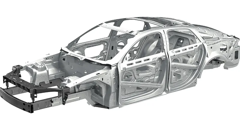
BIW structure of a vehicle

Federal Motor Vehicle Safety Standards (FMVSS) 208

Federal Motor Vehicle Safety Standard (FMVSS) 208 - Occupant Crash Protection establishes performance requirements to determine whether passenger vehicles, light multipurpose vehicles, and trucks meet conditions and injury criteria specified by the standard. This Standard applies to MPVs, trucks and buses, and to vessels designed to contain a pressurized fluid or gas, and to explosive devices for use in the above type of motor vehicles as part of a system designed to provide protection to occupants in the event of a crash. It specifies seat belt types, locations and compatibility with child safety seats, performance requirements and a warning system when the driver’s seat belt is disconnected.

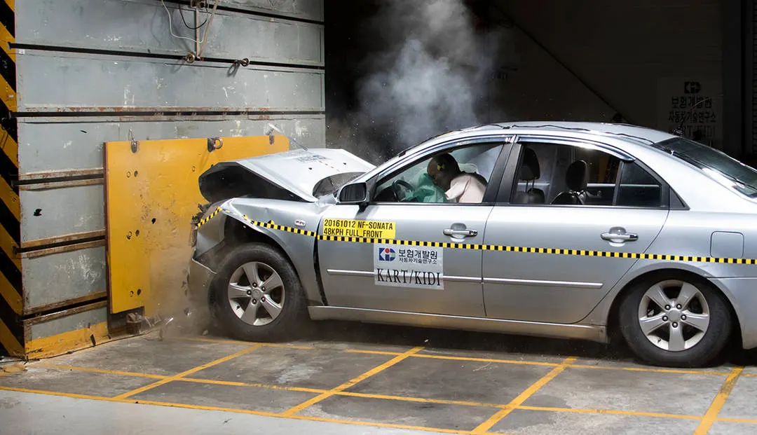
The Full Frontal Fixed Barrier Crash test (or Rigid Barrier test) represents a vehicle-to-vehicle full frontal engagement crash with each vehicle moving at the same impact velocity. A schematic of the test configuration is shown in Figure 2-4. The test is intended to represent most real world crashes (both vehicle-to-vehicle and vehicle-to-fixed object) with significant frontal engagement in a perpendicular impact direction. For FMVSS No. 208, the impact velocity is 0 to 48 kmph (0 to 30 mph), and the barrier rebound velocity, while varying somewhat from car to car, typically ranges up to 10 percent of the impact velocity for a change in velocity of up to 53 kmph. Note that although the rebound velocity varies somewhat from vehicle to vehicle, it is small compared to the impact speed, and the rigid barrier test therefore exposes the belted or unbelted occupant to approximately the same change in velocity (48 kmph plus the rebound velocity) for any vehicle. It is a full systems test which evaluates the protection provided by both the energy-absorbing vehicle structure and the occupant restraint system. Together with performance requirements, it ensures that the vehicle provide the same minimum level of protection in single vehicle crashes also regardless of the vehicles mass or size.

PROCEDURE :

1. Import the given BIW model neon_front_0000.rad using the Import Solver Deck option in RADIOSS.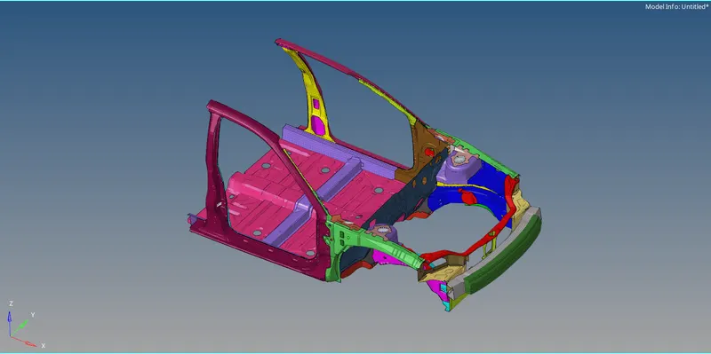

BIW model

2. The given model is checked for unit consistency. In this analysis, [kg mm ms] unit system is followed. For this, the given model file is opened in Notepad and checked as shown below.

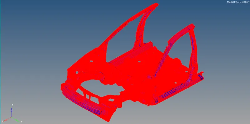
3. As the model is to crash into a rigid wall, appropriate contact interface have to be defined. TYPE7 self contact is defined with co-efficient of friction as 0.2 and other recommended parameters. The entire BIW structure is selected as master surface and the entire nodes as slave nodes as shown below.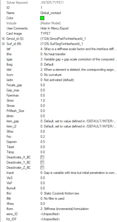

4. Some rigid bodies in the model are having connectivity issues as shown below. It is rectified by updating the connectivity using 1D -> rigids -> update -> connectivity tool.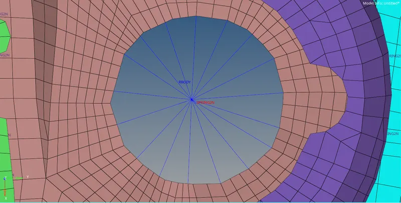

Rigid body error

5. A rigid wall is to be created for the car model to crash into. Rigid wall is created by specifying a base node and the plane normal direction. It is created with co-efficient of friction as 0.1.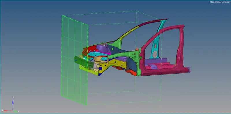

Rigid wall creation

6. As we are dealing with only the front part of the BIW, the total mass of the structure is less than the mass of the complete BIW. Mass plays an important role in the analysis because it determines the kinetic energy of the model under analysis. So, mass have to be added to make the given model behave like the complete BIW model. Mass of the given model is 188 kg. The target mass is 700 kg. Also, mass have to be added in such a way that the centre of gravity (COG) of the model comes at the middle of the crossbeam.

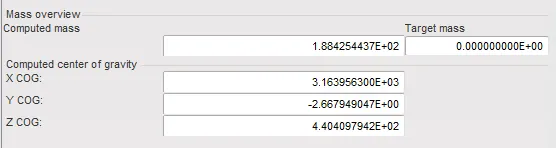
Initial mass

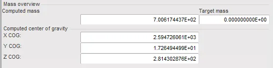
Final mass after mass addition

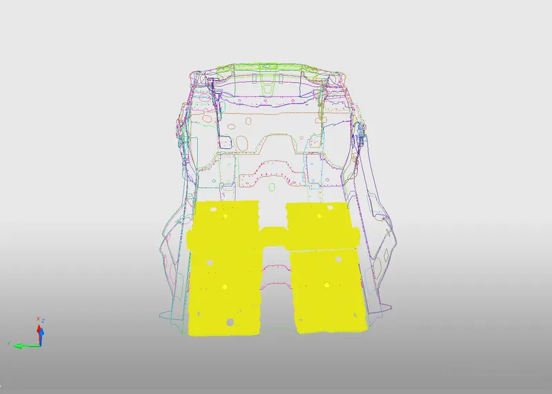
Mass added region

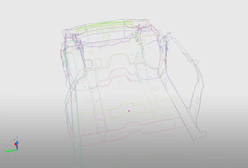
COG after mass addition(pink dot)

7. The entire BIW model have to be given an initial velocity as per the FMVSS criteria , i.e., 35 mph (15.646 mm/ms). It is done by creating INIVEL card and giving the velocity value and select the whole component.

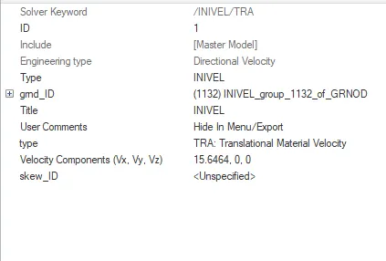
INIVEL card

8. Set the time step to 0.5 microseconds in ENGINE_KEYWORDS -> DT -> DT/NODA.

9. Also, set the simulation run time to 80 ms in ENGINE_KEYWORDS -> RUN -> ENG_RUN.

OUTPUT REQUESTS :

Sectional Force

1. Rail

• Create a local frame at the section where we want to create a section using Solver -> Create -> FRAME -> MOV tool.
• Create a set to store elements at the required section using Model -> Create -> Set tool.
• Now, create a section by calling the local frame and the element set created using Solver -> Create -> SECT tool.

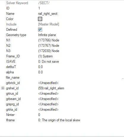
SECT card

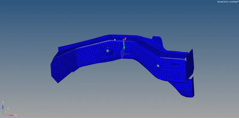
Section created in the rail

• The local sectional force is requested in the Time History file using Solver -> Create -> TH -> /TH/SECTIO card.

2. Shotgun

• Create a local frame at the section where we want to create a section using Solver -> Create -> FRAME -> MOV tool.
• Create a set to store elements at the required section using Model -> Create -> Set tool.
• Now, create a section by calling the local frame and the element set created using Solver -> Create -> SECT tool.

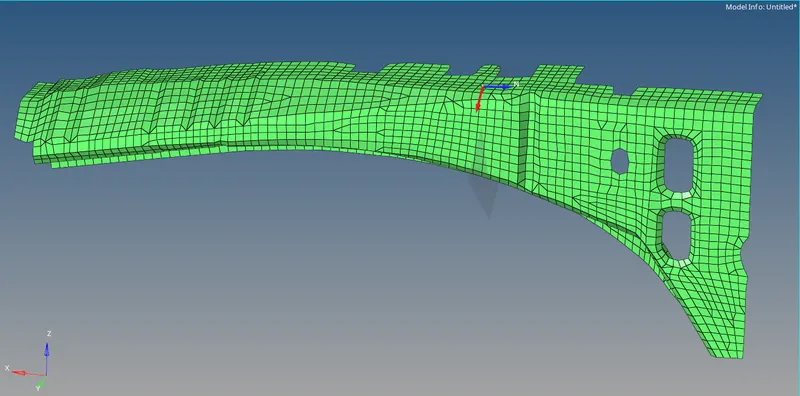
Section created in the shotgun

• The local sectional force is requested in the Time History file using Solver -> Create -> TH -> /TH/SECTIO card.

3. A-pillar

• Create a local frame at the section where we want to create a section using Solver -> Create -> FRAME -> MOV tool.
• Create a set to store elements at the required section using Model -> Create -> Set tool.
• Now, create a section by calling the local frame and the element set created using Solver -> Create -> SECT tool.

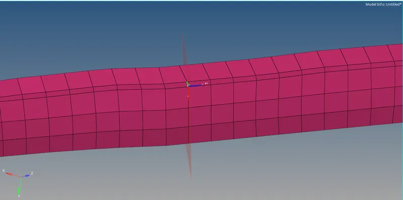
Section created in the A- pillar

• The local sectional force is requested in the Time History file using Solver -> Create -> TH -> /TH/SECTIO card.

Axial force received on the rails from bumper

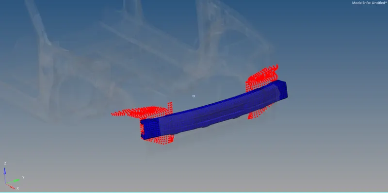
• For axial force on the rail from the bumper, a TYPE7 contact interface is created between the rail and the bumper with bumper as master surface and rail nodes as slave nodes as shown below.

• The interface axial force is requested in the Time history file using Solver -> Create -> TH -> /TH/INTER card.

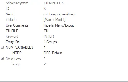
/TH/INTER card

Acceleration of rocker at the base of B-pillar

• For finding the acceleration of the rocker, an accelerometer is fixed on the rocker at the base of B-pillar using Solver -> Create -> ACCEL card and the node is specified where we want to find the acceleration.

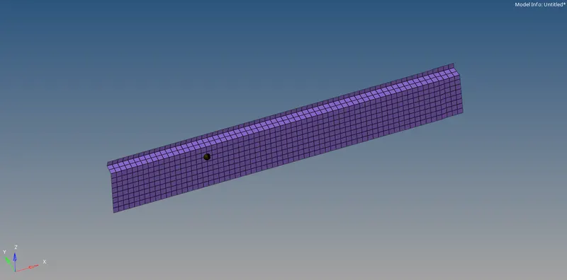
Accelerometer on the rocker

• Acceleration is requested in the Time History file using Solver -> Create -> TH -> /TH/ACCEL card.

Intrusions on the dash wall nodes - 66695,66244

• The given dash wall nodes are shown below.

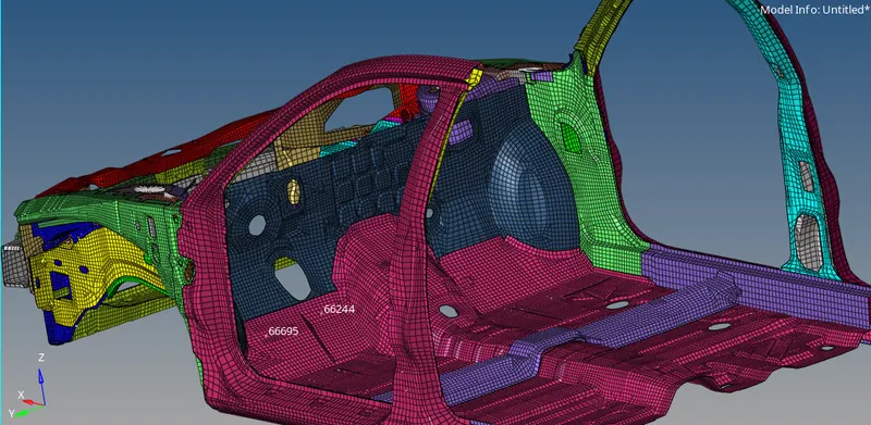
• For finding the intrusions of these nodes, we need to create a local moving frame on the BIW model and the displacement of the nodes is requested in the Time History file using Solver -> Create -> TH -> /TH/NODE card.

Penetration check

• After the model is completely setup, it is checked for any initial penetrations or intersections.
• To check this, go to Penetration Check in Tools tab.
• Both the interfaces created are selected for penetration check.

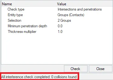
After setting up all the conditions and requesting the required outputs, the model is proceeded to analysis using Analysis -> Radioss option.

RESULTS :

The frontal crash analysis is carried out and the following results are obtained.

Displacement contour plot

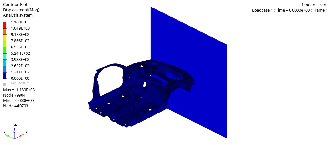
• This contour plot shows the displacement of each node of the BIW model in a graphical interface.
• Displacements are computed with respect to the global co-ordinate system.
• As the model crashes into the rigid wall, deformation occurs to each nodes and the nodes gets displaced from their initial position.
• During the analysis, maximum displacement occured at node 79904 and it got displaced by 1180 mm.

Von-Mises stress contour plot

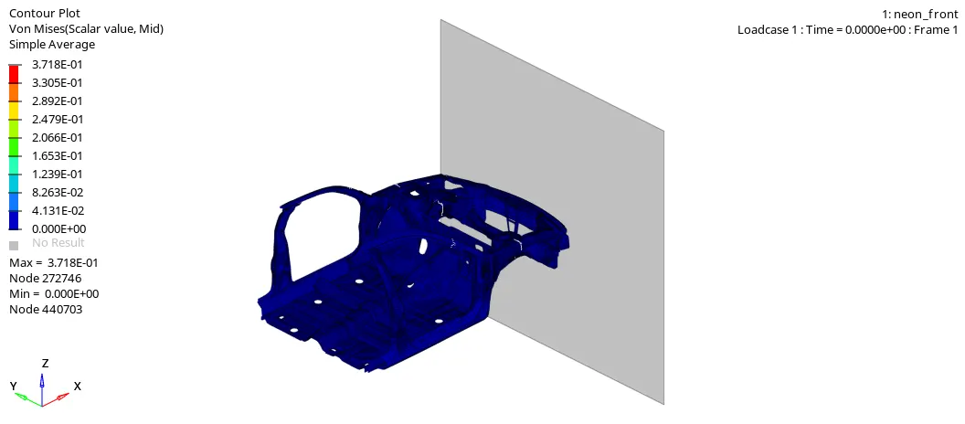
• This contour plot gives the stress induced at each node in the BIW model.
• As the model crashes, internal stress is developed in the model due to material behaviour.
• When the stress developed crosses the yield limit of the material assigned, it undergoes plastic deformation as we can observe from the plot.
• Maximum stress is developed at node 272746 and is equal to 0.3718 GPa.

Axial force received on the rails from the bumper

• We have created a contact interface between the rails and the bumper.
• The contact force between the parts in the global X-direction gives the required axial force. The plot obtained from the Time history is given below.

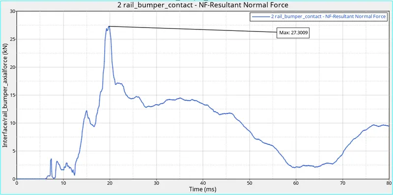
• The contact force is zero till the model touches the rigid wall.
• When the car crashes with the rigid wall, the contact comes into action and the contact force increases as seen from the plot.
• As time proceeds, contact force increases as the bumper undergoes deformation and it reaches a maximum value 27.3009 kN at time 19.8 ms.
• By this time, the force is transferred to other parts of the car and starts to deform. Thus, the contact force between the rail and the bumper reduces after 19.8 ms as seen from the plot.

Sectional forces

NOTE : From here onwards, the rail at the left side of the BIW model when viewed from the front of the car denotes the left rail. Similarly, the rail at the right side of the BIW model when viewed from the front of the car denotes the right rail.(Applicable for shotgun and A-pillar also)

1. Rails (Left and right)

• We have defined sections at both the rails along with a local frame of reference.
• Therefore, the force along the Z- direction of the local frame of reference gives the cross-sectional force in the rails.
• The plot obtained is given below.

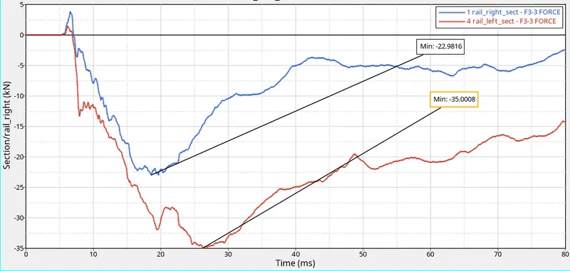
• From the plot, we can see that both the rails are under compression which is obvious.
• From this plot, we can conclude that the force propagation is not same through the left and right rails. It is also clear from the animation file that the deformation is different in left and right side of the car model.
• We can see from the plot that both the plots are decreasing initially, i.e., force is increasing in the negative direction.
• When the compressive force reaches the max. value, bending starts in the rails and starts to deform rapidly. Therefore, the sectional compressive force decreases as seen from the plot.
• The sectional force in the left rail is higher than the right rail throughout the simuation. This is because the transfer of force from the bumper to the left and right rails is not symmetric. Also it depends on the definition and position of the section created as the force being considered here is transfered in all three dimensions.
• The maximum sectional force (compressive) on the left and right rail are 35.0008 kN and 22.9816 kN respectively.

2. Shotgun (Left and right)

• We have defined sections at both the shotguns along with a local frame of reference.
• Therefore, the force along the Z- direction of the local frame of reference gives the cross-sectional force in the shotguns.
• The animation showing the crash of shotgun is given below.

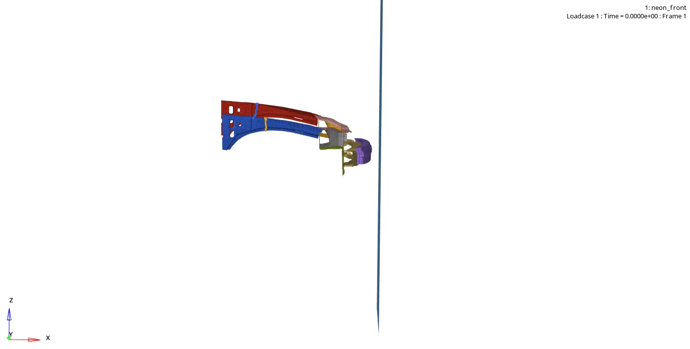
• The plot obtained is given below.

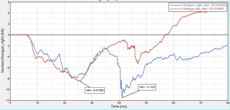
• Initially, both the shotguns are under compression since the bumper undergoes deformation and compressive forces act on the shotguns.
• This compressive force increases and reaches a maximum value. Then the shotguns start to bend and deform plastically which is evident from the animation. During this time, the compressive forces start to decrease.
• As the crash proceeds, the shotguns will come into contact with the rigid wall and the rigid wall exerts force directly on the shotguns which again increases the compressive sectional force.
• As the bending of the shotguns proceed, the sectional compressive force will again start to decrease towards the end of simulation.
• The left shotgun section is under tension at the end of simulation due to excessive bending.
• The maximum sectional force (compressive) on the left and right shotguns are 8.47386 kN and 11.523 kN respectively.

3. A-pillar (left and right)

• We have defined sections at both the A-pillars along with a local frame of reference.
• Therefore, the force along the Z- direction of the local frame of reference gives the cross-sectional force in the A-pillars.
• The plot obtained is given below.

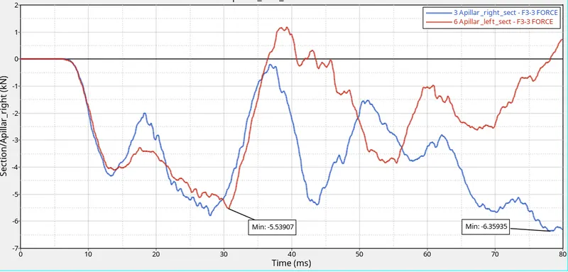
• A-pillars are not undergoing much deformations in this analysis.
• The sectional force in the A-pillars is rapidly varying in nature as is seen from the plot. This is due to the deformation of parts in front of the A-pillars. Due to this, the force transfer is very much irregular.
• The maximum sectional force (compressive) on the left and right A-pillars are 5.53907 kN and 6.35935 kN respectively.

Acceleration of rocker at the base of B-pillar

• We have defined an accelerometer on the rocker at the base of the B-pillar to get the acceleration of the rocker during the simulation.
• The plot obtained is given below.

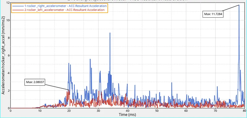
• The rocker is undergoing excessive jerk during the simulation as the acceleration is varying rapidly.
• The maximum acceleration of the left and right rockers are 2.08037 mm/ms2 and 11.7284 mm/ms2 respectively.

Intrusions on the dash wall nodes - 66695,66244

• We have defined a local moving frame at the crossbeam member in order to find out the intrusions of the given nodes.
• The plot obtained is given below.

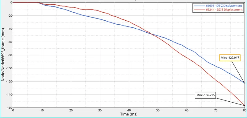
• For measuring intrusions, local moving frame should be used instead of skew.
• Frames give the relative displacement with respect to the moving frame.
• From the above plot, we can find that the node 66695 has intruded 122.947 mm from the position of the node if there were no rigid wall, into the cabin in the local Z-direction at the end of the crash simulation. Similarly. the node 66244 has intruded 156.715 mm into the cabin in the local Z-direction at the end of the simulation.

Energy plot

• The energy plot is given below.

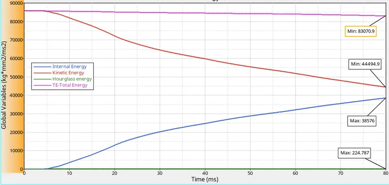
• At the start of the simulation, the car model is possessing only kinetic energy due to the initial velocity boundary condition.
• As the model crashes into the rigid wall, kinetic energy gets converted into internal energy due to plastic deformations happening in the model. Therefore, kinetic energy reduces and internal energy increases during simulation.
• Kinetic energy at the end of the simulation is found to be 44,494.9 kN-mm and the internal energy is 38,576 kN-mm at the end of the simulation.
• Hourglass energy is almost negligible (only 224.787 kN-mm) since we have used QEPH element formulation.
• Since there is not much energy loss, the total energy remains almost constant throughout the simulation.

Checking mass and energy error

• After simulation, the Engine OUT file is opened in Notepad and checked for mass and energy error.

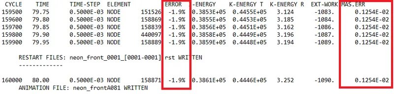
• The energy error after simulation is -1.9% and the mass error is 0.001254% which are well within the limits.

CONCLUSION :

The frontal crash analysis is done on the given Dodge Neon BIW model and the results are analysed. Crashworthiness analysis is mainly carried out to determine whether a car is safe to run in a particular road condition. There are different standards of conducting the crash analyses. The one which is followed in this project is FMVSS 208 standards.These tests are conducted to determine

• how much internal energy the vehicle is able to absorb during a crash
• the deformations occured in certain critical areas
• the occupant safety

These parmeters are then compared with the Standards and finally decide which level of safety category the particular vehicle fits into.