Week - 9 Material Modeling from Raw Data

AIM :

To model an elasto-plastic material using MAT_024 or MAT_018 material model from the given True Stress-Strain data and verify it by conducting a tensile test simulation on the Dog-Bone specimen.

TOOLS REQUIRED :

• LS-PrePost
• LS-Run
• MS-Excel

INTRODUCTION :

Material deformation can be permanent or temporary. Permanent deformation is irreversible i.e. stays even after removal of the applied forces, while the temporary deformation disappears after removal of the applied forces i.e., the deformation is recoverable. Both kinds of deformation can be function of time, or independent of time. Temporary deformation is called elastic deformation, while the permanent deformation is called plastic deformation. Time dependent recoverable deformation under load is called anelastic deformation, while the characteristic recovery of temporary deformation after removal of load as a function of time is called elastic aftereffect. Time dependent i.e. progressive permanent deformation under constant load/stress is called creep. For viscoelastic materials, both recoverable and permanent deformations occur together which are time dependent. When a material is subjected to applied forces, first the material experiences elastic deformation followed by plastic deformation. Extent of elastic and plastic deformations will primarily depend on the kind of material, rate of load application, ambient temperature, among other factors. Change over from elastic state to plastic state is characterized by the yield strength (`sigma_0`) of the material.

Forces applied act on a surface of the material, and thus the force intensity, force per unit area, is used in analysis. Analogous to this, deformation is characterized by percentage change in length per unit length in three distinct directions. Force intensity is also called engineering stress (or simply stress, s), is given by force divided by area on which the force is acting. Engineering strain (or simply strain, e) is given by change in length divided by original length. Engineering strain actually indicates an average change in length in a particular direction. According to definition, s and e are given as

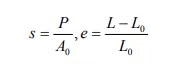
where P is the load applied over area `A_0`, and as a consequence of it material attains the final length `L` from its original length of `L_0`.

Because material dimensions changes under application of the load continuously, engineering stress and strain values are not the true indication of material deformation characteristics. Thus the need for measures of stress and strain based on instantaneous dimensions arises. Ludwik first proposed the concept of, and defined the true strain or natural strain (`epsilon`) as follows:

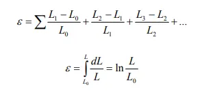
As material volume is expected to be constant i.e. `A_0L_0=AL`, and thus

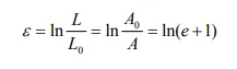
There are certain advantages of using true strain over conventional strain or engineering strain. These include (i) equivalent absolute numerical value for true strains in cases of tensile and compressive for same intuitive deformation and (ii) total true strain is equal to the sum of the incremental strains.

True stress (σ) is given as load divided by cross-sectional area over which it acts at that instant.

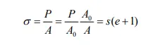
It is to be noted that engineering stress is equal to true stress up to the elastic limit of the material. The same applies to the strains. After the elastic limit i.e. once material starts deforming plastically, engineering values and true values of stresses and strains differ.
The above equation relating engineering and true stress-strains are valid only up to the limit of uniform deformation i.e. up to the onset of necking in tension test. This is because the relations are developed by assuming both constancy of volume and homogeneous distribution of strain along the length of the tension specimen.

Elastic deformation

Elastic deformation is reversible i.e. recoverable. Up to a certain limit of the applied stress, strain experienced by the material will be the kind of recoverable i.e. elastic in nature. This elastic strain is proportional to the stress applied. The proportional relation between the stress and the elastic strain is given by Hooke’s law, which can be written as follows:

where the constant E is the modulus of elasticity or Young’s modulus,

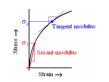
Though Hooke’s law is applicable to most of the engineering materials up to their elastic limit, defined by the critical value of stress beyond which plastic deformation occurs, some materials won’t obey the law. E.g.: Rubber, it has non-linear stress-strain relationship and still satisfies the definition of an elastic material. For materials without linear elastic portion, either tangent modulus or secant modulus is used in design calculations. The tangent modulus is taken as the slope of stress-strain curve at some specified level, while secant modulus represents the slope of secant drawn from the origin to some given point of the σ-ε curve, as shown in the fig. below.

If one dimension of the material changed, other dimensions of the material need to be changed to keep the volume constant. This lateral/transverse strain is related to the applied longitudinal strain by empirical means, and the ratio of transverse strain to longitudinal strain is known as Poisson’s ratio (`nu`). Transverse strain can be expected to be opposite in nature to longitudinal strain, and both longitudinal and transverse strains are linear strains. For most metals the values of `nu` are close to 0.33, for polymers it is between 0.4 – 0.5, and for ionic solids it is around 0.2.

Plastic deformation

When the stress applied on a material exceeds its elastic limit, it imparts permanent non-recoverable deformation called plastic deformation in the material. Microscopically it can be said of plastic deformation involves breaking of original atomic bonds, movement of atoms and the restoration of bonds i.e. plastic deformation is based on irreversible displacements of atoms through substantial distances from their equilibrium positions. The mechanism of this deformation is different for crystalline and amorphous materials. For crystalline materials, deformation is accomplished by means of a process called slip that involves motion of dislocations. In amorphous materials, plastic deformation takes place by viscous flow mechanism in which atoms/ions slide past one another under applied stress without any directionality.

Plastic deformation is, as elastic deformation, also characterized by defining the relation between stresses and the corresponding strains. However, the relation isn’t simpler as in case of elastic deformation, and in fact it is much more complex. It is because plastic deformation is accomplished by substantial movement of atomic planes, dislocations which may encounter various obstacles. This movement becomes more complex as number slip systems may get activated during the deformation.

The analysis of plastic deformation, and the large plastic strains involved is important in many manufacturing processes, especially forming processes. It is very difficult to describe the behavior of metals under complex conditions. Therefore, certain simplifying assumptions are usually necessary to obtain an amenable mathematical solution. Important assumptions, thus, involved in theory of plasticity are neglecting the following aspects:

(i) Anelastic strain, which is time dependent recoverable strain.
(ii) Hysteresis behavior resulting from loading and un-loading of material.
(iii) Bauschinger effect – dependence of yield stress on loading path and direction

The relations describing the state of stress and strain are called constitutive equations because they depend on the material behavior. These relations are applicable to any material whether it is elastic, plastic or elastic-plastic. Hooke’s law which states that strain is proportional to applied stress is applicable in elastic range where deformation is considered to be uniform. However, plastic deformation is indeed uniform but only up to some extent of strain value, where after plastic deformation is concentrated, the phenomenon called necking. The change over from uniform plastic deformation to non-uniform plastic deformation is characterized by ultimate tensile strength (`sigma_u`). As a result of complex mechanism involved in plastic deformation and its non-uniform distribution before material fractures, many functional relations have been proposed to quantify the stress-strain relations in plastic range.

A true stress-strain relation plotted as a curve is known as flow curve because it gives the stress (σ) required to cause the material to flow plastically to any given extent of strain (ε) under a set of conditions. Other important parameters affecting the stress-strain curve are : rate at which the load is applied / strain rate (`epsilon^.`), and the temperature of the material (T, in K) i.e.,

Following are the most common equations that describe the material flow behavior:

where K is strength coefficient, and n is strain hardening exponent. The strain-hardening exponent may have values from n=0 (perfectly plastic solid) to n=1 (elastic solid). For most metals, n has values between 0.10 and 0.50. The Power law equation described above is also known as Holloman-Ludwig equation.

Another common variation from Power law equation, also known as Ludwig equation, is:

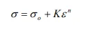
where `sigma_0` is the yield strength of the material.

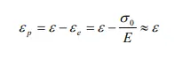
Many other expressions for flow curve are available in literature. The true strain used in the above equations should actually be the effective plastic strain value, given by the following equation, where elastic strains can be safely neglected because plastic strains are very much when compared with elastic strain values.

PROCEDURE :

NOTE : (kg.mm,ms) unit system is followed consistently throughout the whole study.

• The material curve for which the material model has to created is shown below.

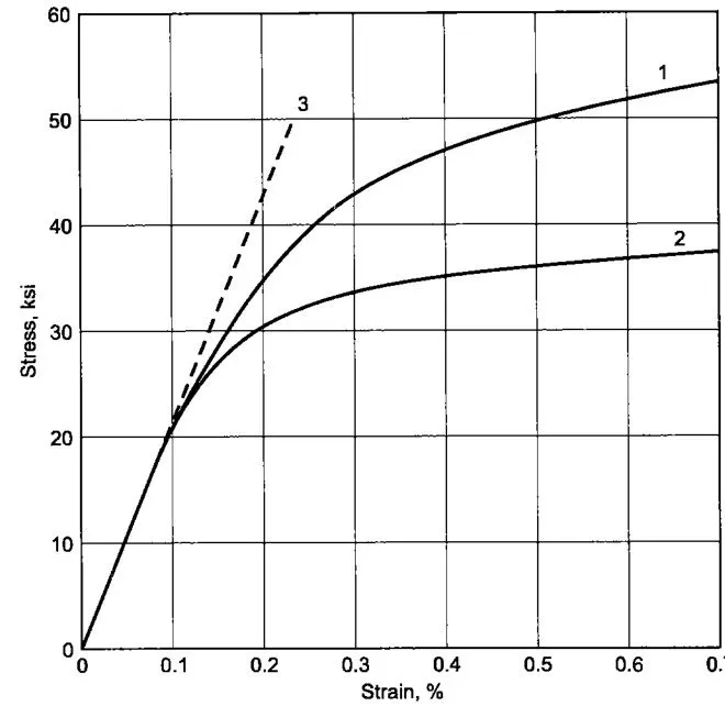
True Stress-Strain curve

• The curve number 2 is selected from the figure for material modelling and MAT_024 model is used for creating the material card.
• The true stress-strain data is extracted through data digitizer tool and imported into MS-Excel. The extracted stress (ksi) and strain(%) is converted into stress(GPa) and strain(-).
• True Stress-Strain data is plotted in Excel which is shown below.

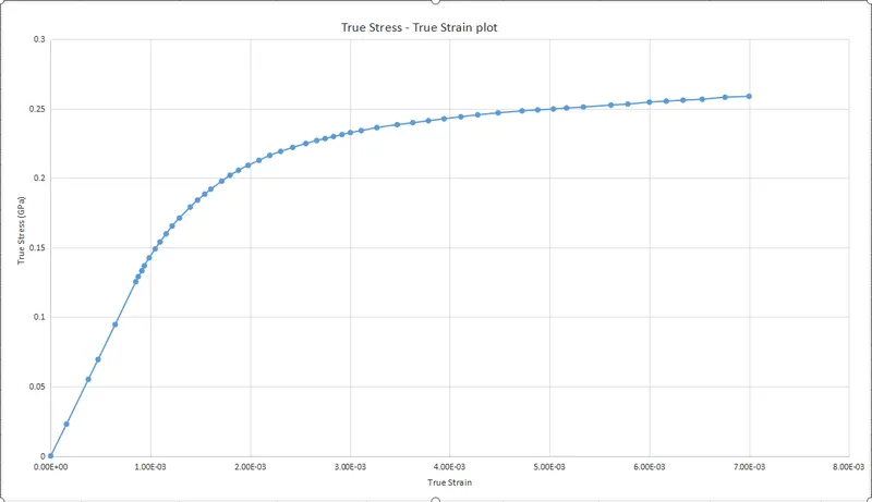
True Stress-Strain plot

• The linear elastic region of the curve is plotted separately to calculate the Young's Modulus.

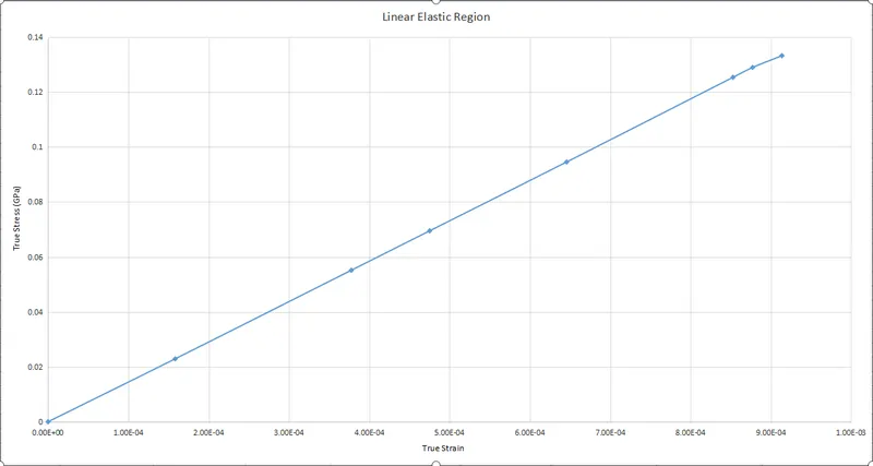
• From the linear elastic region, Young's Modulus is found to be 145.85 GPa.
• Now, the True Stress-Strain data is converted into Effective Stress-Effective Plastic Strain data to find out the yield point of the material. The linear region of the True Stress-Strain plot is perfectly elastic and does not show plastic strain. So, in the Effective Stress-Effective Plastic Strain plot, we will see zero strain in the elastic region upto the yield point. From the yield point, it will show plastic strain. Therefore, the first point which shows strain in Effective Stress-Effective Plastic Strain plot is chosen as the yield point of the material.

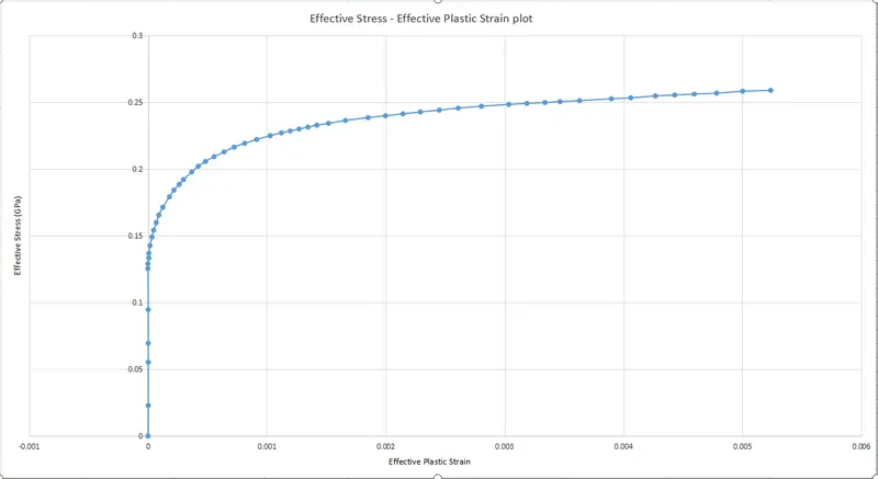
Effective Stress-Effective Plastic Strain plot

• From the above plot, the yield point was found to be at (9.14E-04, 0.1332 GPa). So, the Yield Stress is found to be 0.1332 GPa.
• The hardening curve which is to be defined in the material card should start ideally with yield point.
• Therefore, the Effective Stress-Effective Plastic Strain plot starting from the yield point is plotted and is shown below.

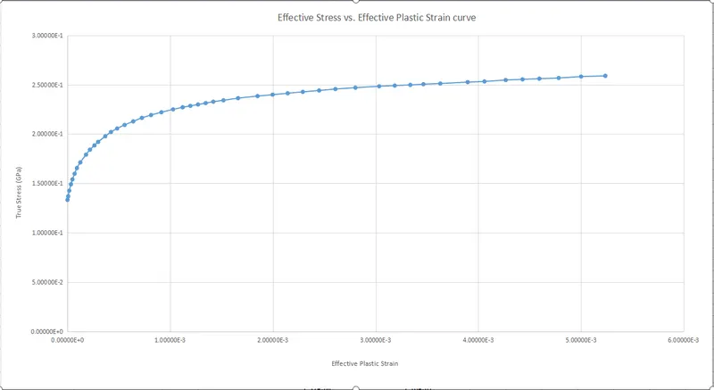
Hardening curve plot (starting from Yield point)

• The above data is to be entered into the MAT_024 material model through LCSS option.
• First, the data is input as a curve using *DEFINE_CURVE keyword as shown below.

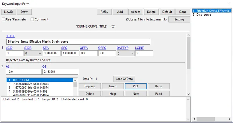
Defining the hardening curve

• *MAT_PIECEWISE_LINEAR_PLASTICITY (MAT_024) material card is defined with the data (Young's Modulus, Yield Stress, and Effective Stress-Effective Plastic Strain curve) extracted from the given material data.
• Density and Poisson's ratio data are taken from the Gray Cast Iron material data.

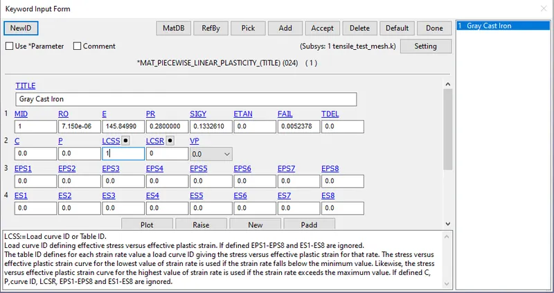
Defining MAT_024 material model

• The Dog-Bone specimen is opened in LS-PrePost for verification of the modelled material card.

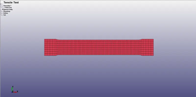
Dog-Bone 2D specimen

• The section properties for the Dog-Bone are defined by using *SECTION_SHELL keyword. All the properties are set to default and a thickness of 2.67mm is assigned to the shell elements.

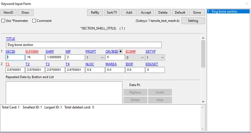
Section definition for the Dog-Bone part

• The modelled material card and section is assigned to the Dog-Bone specimen in *PART keyword.

• Next, the specimen has to be constrained by giving proper boundary conditions.
• One end of the specimen has to be constrained similar to how it is held in the chuck of the UTM.
• The centre nodes on the fixed end of the specimen are constrained in translation and rotation in and about every axis as shown below.

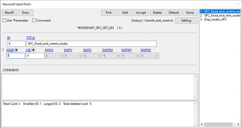
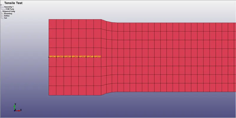
SPC on the centre nodes of fixed end

• Remaining nodes on the fixed end are constrained in translation and rotation in and about every axis except translation in Y-direction as the specimen compression along Y-direction due to Poisson effect.

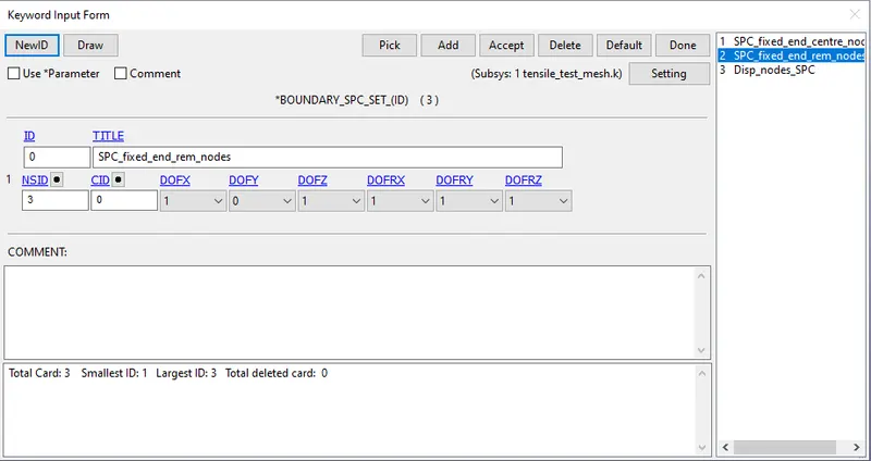
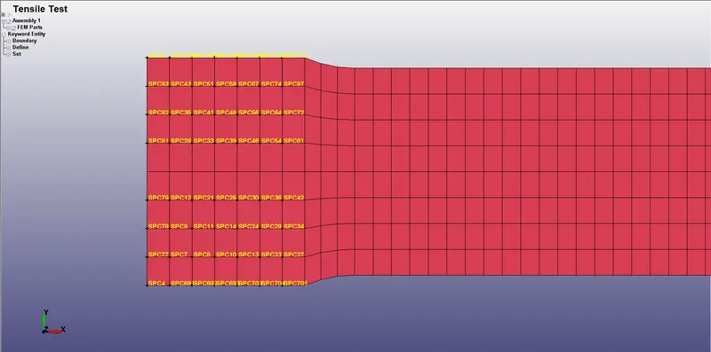
SPC on the remaining nodes of fixed end

• All the nodes on the moving end are constrained in translation and rotation in and about every axis except translation in X-direction.

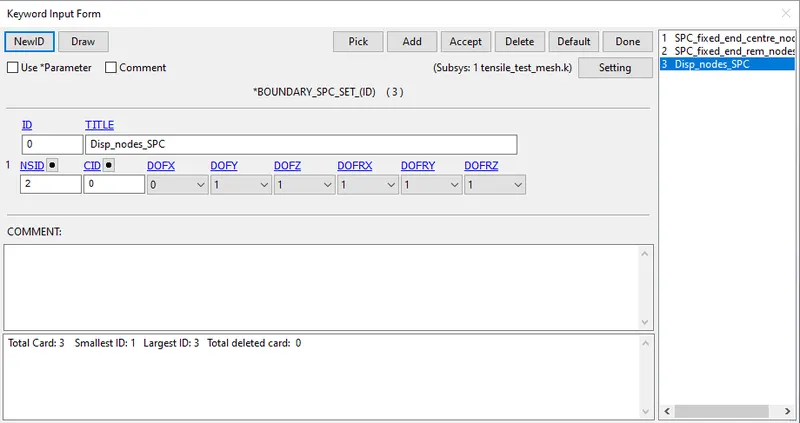
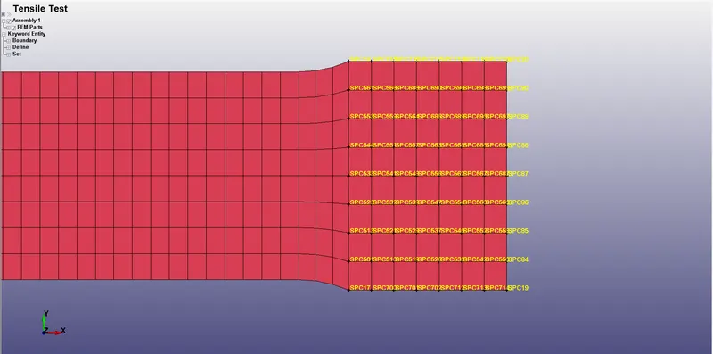
SPC on the nodes of moving end

• Displacement boundary condition is given to the nodes on the moving end using *BOUNDARY_PRESCRIBED_MOTION_SET keyword as shown below.

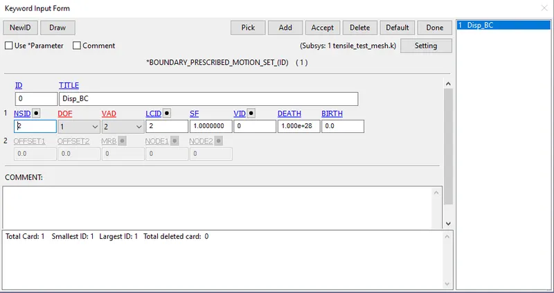
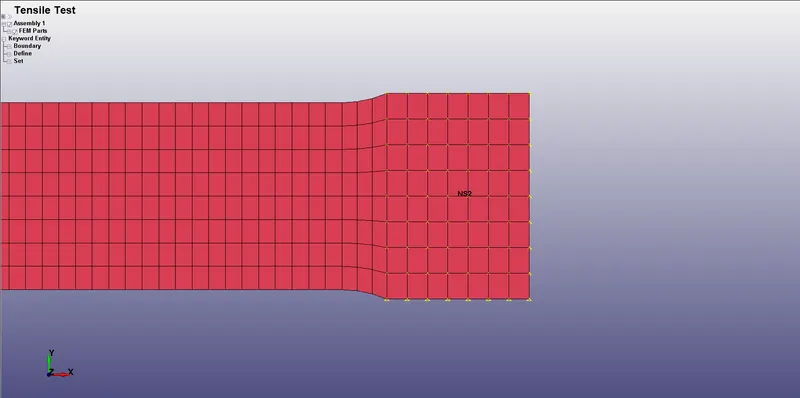
Prescribed motion BC on the nodes of moving end

• Displacement is applied at a constant rate and a displacement of 0.6 mm is given to the specimen. The load curve is shown below.

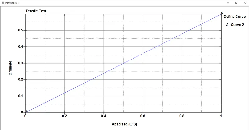
Load curve defining the displacement BC

• The tensile test is conducted at a low strain rate without allowing the system to experience any inertial effects. So, the tensile test is actually a static non-linear (material and geometric non-linearity) problem physically.
• Therefore, Implicit solver should be used to solve this problem.
• Implicit method is activated by using *CONTROL_IMPLICIT_GENERAL keyword. The IMFLAG parameter is switched to 1 to activate the implicit method. All other options are set to default.

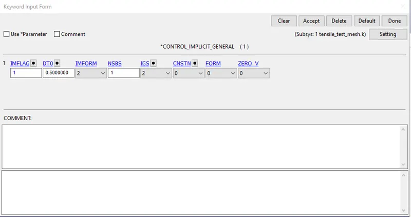
• Another keyword *CONTROL_IMPLICIT_AUTO is used which controls the time step size for the problem. Auto-time stepping option is used with IAUTO parameter which will alter the time step size depending upon the number of equilibrium iterations solved within every time step. No. of Equilibrium iterations is set to 11 and iteration window is set to 5 which is the default.

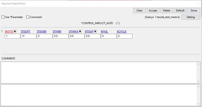
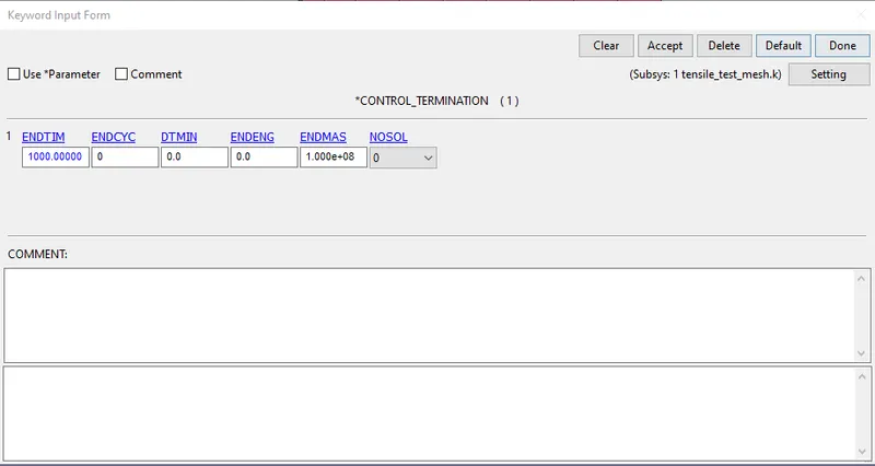
• The termination time for the simulation is set to 1000 ms in the *CONTROL_TERMINATION card as shown below.

• At last, the required outputs should be requested using *DATABASE card.
  
  • *DATABASE_BINARY_D3PLOT - Animation file is requested using this card.
  • *DATABASE_EXTENT_BINARY - Strain data are written to the animation d3plot file using this card.

RESULTS AND DISCUSSIONS :

X-Stress contour plot

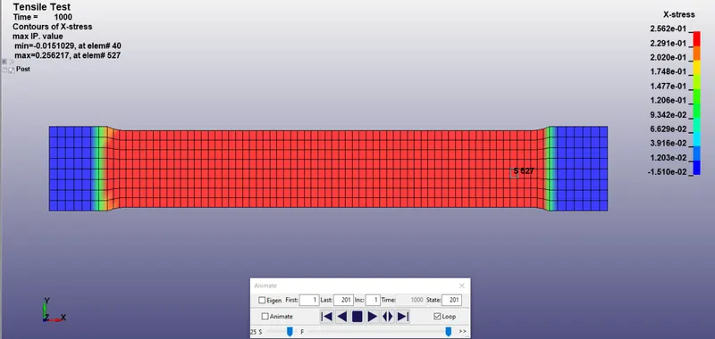
• The figure below shows the X-Stress contour when the specimen is in tension.

X-Stress contour plot

• We can observe a max. X-stress of 0.256 GPa at element number 527 which is in the range of the input data, so that we can assure that the solver didn't extrapolate beyond the range of input data.

Effective Plastic Strain contour plot

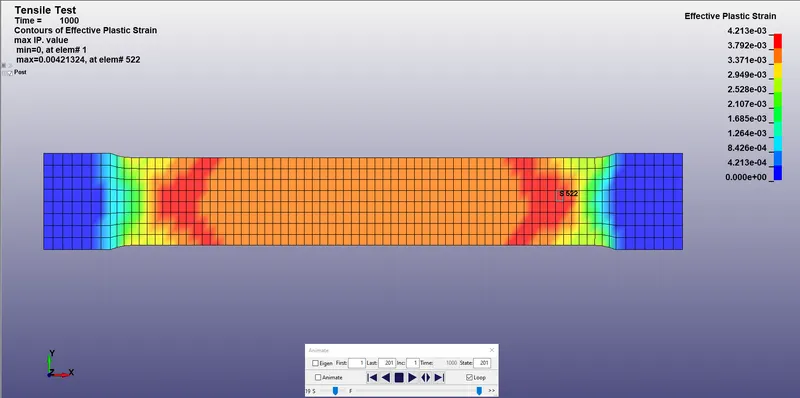
• The figure below shows the Effective Plastic Strain contour when the specimen is in tension.

Effective Platic Strain contour plot

• We observe a max. Effective Plastic Strain of 4.213E-03 at element number 522 which is also in the range of the input data provided in the material model, as expected.

Material model verification

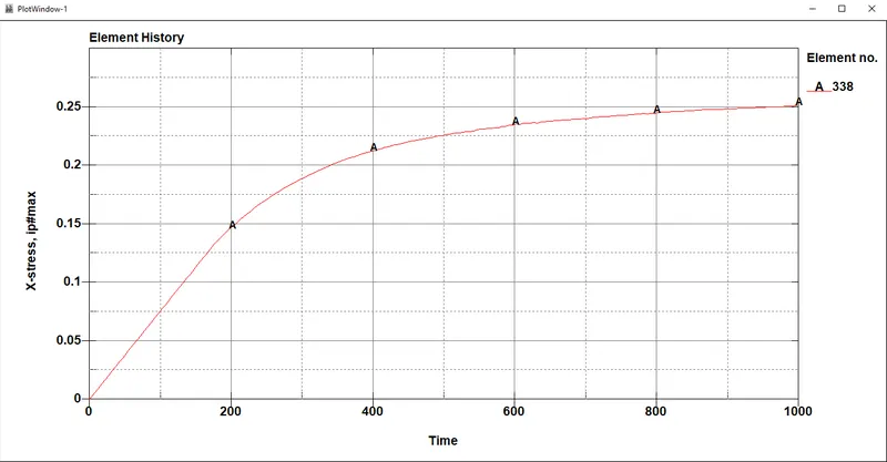
• The plot below depicts the X-Stress behaviour of an element in the middle portion of the specimen with respect to the simulation time.

X-Stress vs. Time plot

• The stress value is going above the yield stress value, so there would be plastic deformation in the model.

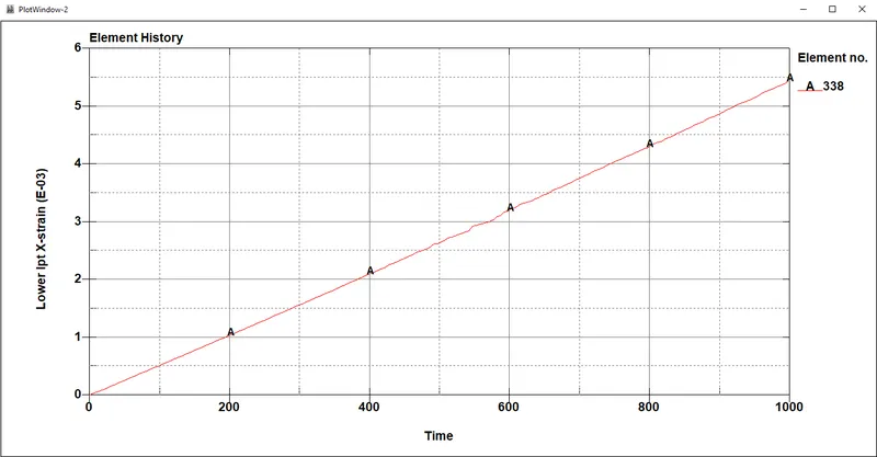
• The plot below depicts the X-strain behaviour of the same element with respect to the simulation time.

X-Strain vs. Time plot

• To verify the material model, we should compare the True Stress vs. True Strain plot from the simulation with the same plot which is used to model the material.
• True Stress vs. True Strain plot from the simulation is extracted from the Element history data by cross-plotting X-stress vs. Time and X-strain vs. Time plots.

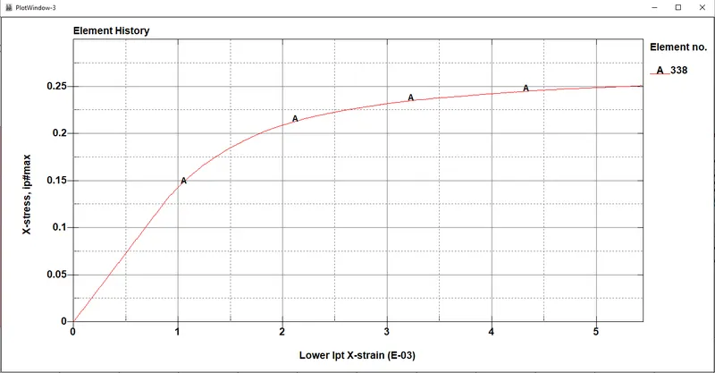
X-stress vs. X-strain plot (by cross-plotting)

• 100 data points are extracted from this plot in .txt file format and this data is imported into MS-Excel.
• The obtained data from the simulation is True stress-strain and the input data used to model the material is also the true stress-strain data. Therefore, no conversion is needed and both the results can be directly compared.
• The data obtained from the simulation is plotted along with the input Stress-Strain data in Excel to compare and verify how the material behaved in the tensile test simulation.

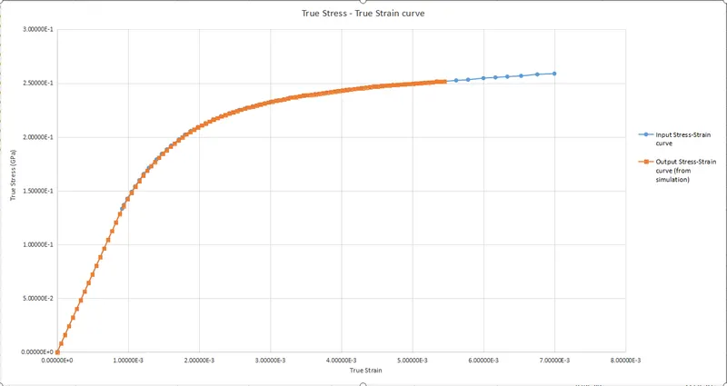
Verification of the MAT_024 material model

• It is observed from the plot that both the curves match each other upto a great extend which means that the material is modelled accurately to the given input curve.
• Young's Modulus is calculated from the simulation True stress-strain data to compare it with the given Young's Modulus value.

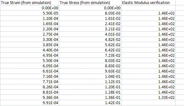
Young's Modulus verification (from simulation data)

• From the simulation, Young's Modulus value obtained is 146 GPa which is very much close to the input value 144 GPa (20.9E+06 psi).

• Similarly, Yield Stress value is also verified through the data extracted from the X-stress vs. Effective Plastic Strain data from the simulation.

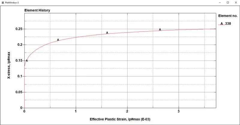
X-stress vs. Effective Plastic Strain plot

• Data points are extracted from the plot and opened in Notepad as shown below.

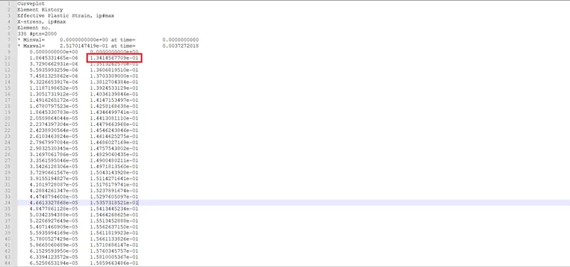
• From the above data, we can observe that the plastic deformation (plastic strain) begins at a stress value of 0.134 GPa which is the Yield stress value obtained from the tensile test simulation.
• This Yield stress value from the simulation is very much close to the value calculated from the input Stress-strain curve, which is 0.133 GPa.
• This shows that Yield stress value is also verified and found to be accurately modelled.

CONCLUSION :

The modelled MAT_024 material card is verified with the given True stress-strain curve. The Stress-strain behaviour after yielding is considered by a hardening curve which is given as an input through MAT_024 card. The MAT_024 material model captures the actual stress-strain behaviour exactly upto a great extend with high level of accuracy.