Week 9 - Parametric study on Gate valve.

• Aim:

To perform a parametric study on the gate valve simulation by setting the opening from 10 % to 80%.

• Objective:

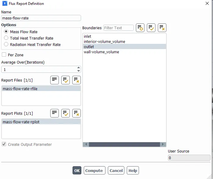
1. Obtain the mass flow rates at the outlet for each design point.
2. Calculate the flow coefficient and flow factor for each opening and plot the graph.
3. Discuss the results of the mass flow rate and flow coefficient.

• Theory:

1. Parametric study:

A parametric study in Simulation is done to Map the change in inputs to the corresponding outputs. As long as the input parameter and output parameters are connected, the corresponding output values for change in input values are obtained.

1. A parametric simulation analysis traces the transition in inputs to the corresponding outputs.
2. Input parametric point and output parametric cases are always connected.
3. If we change the input design points, automatically output value changes.
4. In this case, the process begins with the creation of an input parameter group in the Spaceclaim window. The corresponding parameterized output is the mass flow rate.

2. Gate Valve:

A gate valve, also known as a sluice valve, is a valve that opens by lifting a barrier (gate) out of the path of the fluid. Gate valves require very little space along the pipe axis and hardly restrict the flow of fluid when the gate is fully opened. The gate faces can be parallel but are most commonly wedge-shaped (in order to be able to apply pressure on the sealing surface).

Construction:

Common gate valves are actuated by a threaded stem that connects the actuator (e.g. handwheel or motor) to the gate. They are characterized as having either a rising or a non-rising stem, depending on which end of the stem is threaded. Rising stems are fixed to the gate and rise and lower together as the valve is operated, providing a visual indication of valve position. The actuator is attached to a nut that is rotated around the threaded stem to move it. Non-rising stem valves are fixed to, and rotate with, the actuator, and are threaded into the gate. They may have a pointer threaded onto the stem to indicate valve position since the gate's motion is concealed inside the valve. Non-rising stems are used where vertical space is limited.

Use:

Gate valves are used to shut off the flow of liquids rather than for flow regulation. When fully open, the typical gate valve has no obstruction in the flow path, resulting in very low flow resistance. The size of the open flow path generally varies in a nonlinear manner as the gate is moved. This means that the flow rate does not change evenly with stem travel. Depending on the construction, a partially open gate can vibrate from the fluid flow.

Gate valves are mostly used with larger pipe diameters (from 2" to the largest pipelines) since they are less complex to construct than other types of valves in large sizes.

3. Mass flow rate:

The mass flow rate is the mass of a liquid substance passing per unit time. In other words, the mass flow rate is defined as the rate of movement of liquid pass through a unit area. The mass flow is directly dependent on the density, velocity of the liquid, and area of cross-section. It is the movement of mass per unit time. The mass flow is denoted by m and the units in kg/s.

The mass flow formula is given by,

`m=rho*V*A`

`rho` = density of fluid,

V = velocity of the liquid, and

A = area of cross-section

4. Flow co-efficient:

The flow coefficient of a device is a relative measure of its efficiency at allowing fluid flow. It describes the relationship between the pressure drop across an orifice valve or other assembly and the corresponding flow rate.

Mathematically the flow coefficient C_v (or flow-capacity rating of the valve) can be expressed as :

`C_v=Qsqrt((SG)/(DeltaP)`

where:

Q is the rate of flow (expressed in US gallons per minute),

SG is the specific gravity of the fluid (for water = 1),

ΔP is the pressure drop across the valve (expressed in psi)

In more practical terms, the flow coefficient C_v is the volume (in US gallons) of water at 60 °F that will flow per minute through a valve with a pressure drop of 1 psi across the valve.

The use of the flow coefficient offers a standard method of comparing valve capacities and sizing valves for specific applications that are widely accepted by the industry. The general definition of the flow coefficient can be expanded into equations modeling the flow of liquids, gases, and steam using the discharge coefficient.

For gas flow in a pneumatic system, the C_v for the same assembly can be used with a more complex equation. Absolute pressures (psi) must be used for gas rather than simply differential pressure.

For airflow at room temperature, when the outlet pressure is less than 1/2 the absolute inlet pressure, the flow becomes quite simple (although it reaches sonic velocity internally). With C_v = 1.0 and 200 psi inlet pressure, the flow is 100 standard cubic feet per minute (scfm). The flow is proportional to the absolute inlet pressure, so the flow in scfm would equal the C_v flow coefficient if the inlet pressure were reduced to 2 psi and the outlet was connected to a vacuum with less than 1 psi absolute pressure (1.0 scfm when C_v = 1.0, 2 psi input).

Flow factor:

The metric equivalent flow factor (K_v; commonly used everywhere else in the world with the exception of the United States) is calculated using metric units :

`K_v=Qsqrt((SG)/(DeltaP)`

where

K_v is the flow factor (expressed in )

Q is the flow rate (expressed in cubic meters per hour []),

SG is the specific gravity of the fluid (for water = 1),

∆P is the differential pressure across the device (expressed in [bar]).

K_v can be calculated from C_v using the equation:

`K_v=0.865*C_v*K_v`

• Content:

1. Procedure of simulation:

1. To begin the simulation process open the Workbench > select Fluent Module.
2. Click on Geometry to open SpaceClaim. In SpaceClaim > Import Geometry.
3. Initially perform the analysis without the parametric study as a reference simulation.
4. For this, we give a rise of 10mm for the Gate disc.
5. To visualize clear visualization of Gate disk > unselect the Bottom casing.
6. Now, in Edit > select the Move option > click on Select Component (to select entire Gate disk component) > by clicking Move the gate disk and enter the lift value as 10mm. To parameterize select 'P'.
7. To extract the Fluid volume go to Prepare > select Volume Extract > and use Select Edges > now select Inlet, Outlet and other Edge of fluid volume are below the Bonnet i.e. untick the Bonnet to visualize the edge and select the third Edge > click Ok.
8. After this we need to extend the fluid flow regions i.e. select Pull tool > select the surface of inlet and pull it out and enter the value as 800mm > similarly on the outlet side also.
9. Now Uncheck and Suppress all the solid geometries one by one. See that only Fluid Volume exists. Close SpaceClaim.
10. Open the Meshing Module > check if the Fluid volume is loaded successfully.
11. Generate a baseline mesh for the imported geometry.
12. Assign the Named Selection i.e Inlet and Outlet. Then close the Meshing module and Update the Mesh.
13. Further to proceed with the simulation > open Fluent(Setup). Here use Double Precision with four processors for fast calculations.
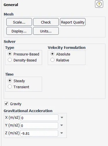
14. To set up the case, unable Gravity. In this case, z-direction is pointing upwards. Hence z=-9.81. For this case consider Solver > Time = steady-state, Type = Pressure Based and Velocity Formulation = Absolute.
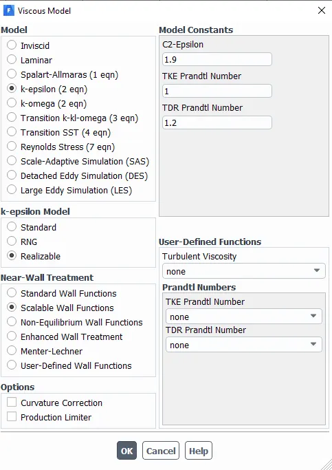
15. Go to Physics > select Viscous Model= k-epsilon model, Realizable, Scalable Wall Functions > click Ok.
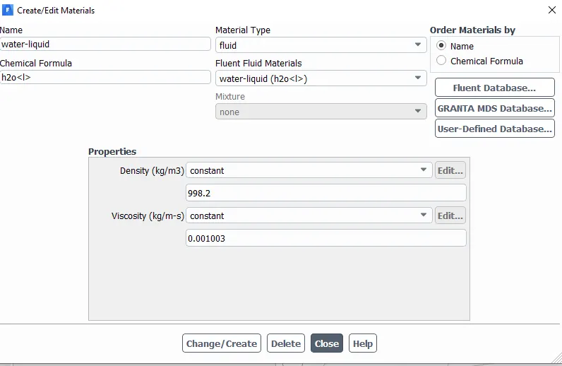
16. To define the Material go to Setting Up Physics > Materials > go to Fluent Database > select Water-Liquid > click on Copy > Close.
17. Now we should define the fluid that is existing inside the Fluid Volume. For this go to Zones > Cell Zones > select Volume > edit Material Name = Water-Liquid > click Ok.
18. To protect the mixing of fluids, go to Materials > go to Fluent-Fluid Materials > delete Air > click Close.
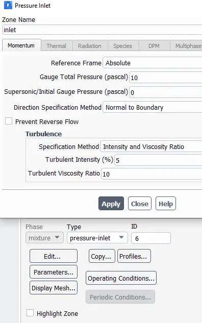
19. Now go to Boundary Conditions > select Inlet > Type=pressure-inlet > select Guage Toatal Pressure=10 pascal > click Ok.
20. Before Initialization, go to Initiallization > select Method=Standard > then go to Options > Solution Initialization page opens > here select compute from= Inlet > now Initialize(t=0).
21. After this, go to Postprocessing > create a plane > in order to view the velocity magnitude- create a contour > click OK.

For the parametric study,

1. As we selected Parametric while entering the lift, just below the Results we can find Parameter set is created.
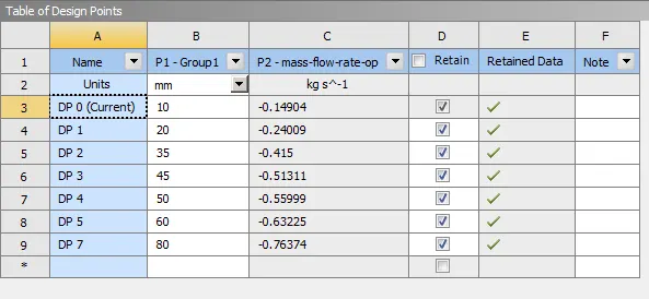
2. Click Parameters to open > we can see the Table of Design Points > we have 3 columns i.e. Name, GROUP-1(p1) and mass flow rate-report (p2).
3. Enter the value of lift required in column-Group1 in column sequence i.e 10% - 80%.
4. In order to calculate all the cases > click on Update All Design Points. Once the calculation starts the values of mass flow rate are displayed in the report (p2).
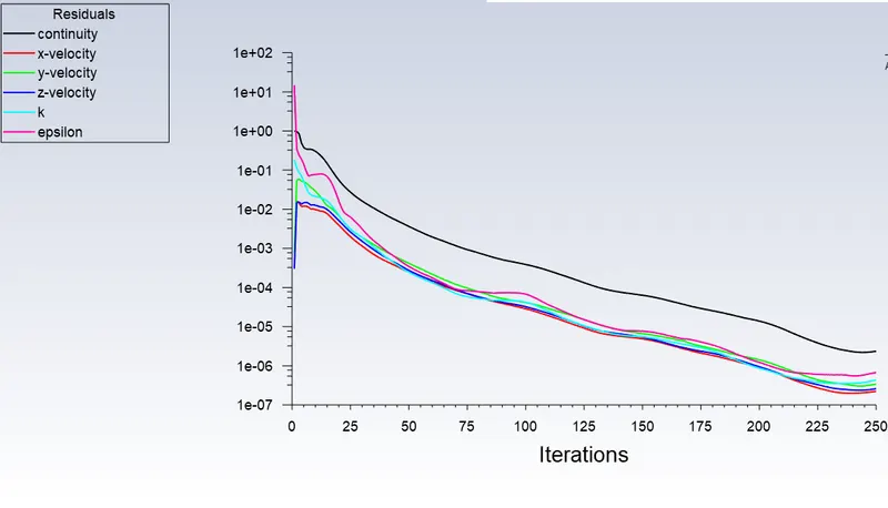
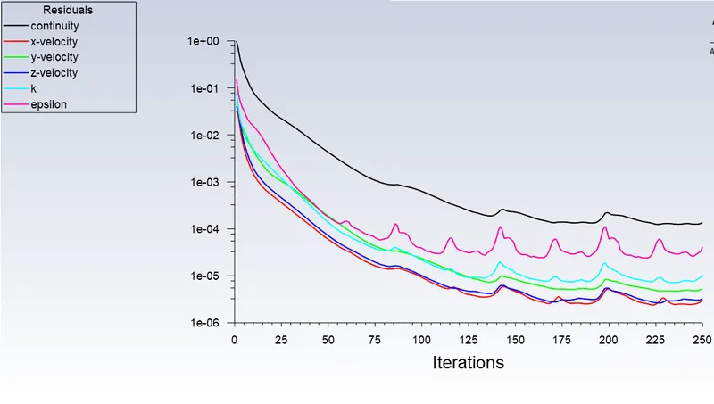
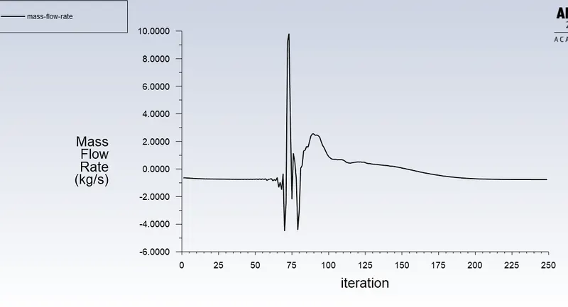
5. If we get any wrong value in mass flow rate, then check the generated residuals and reduce the momentum value and run the calculation only for that particular case. Here to open the particular case, just right click on the case > click Set as Current. Then we can access those particular cases.
6. Finally, residuals, report for the mass flow rate is generated and velocity magnitude is visualised. On generating the data plots are plotted as required.

2. Geometry:

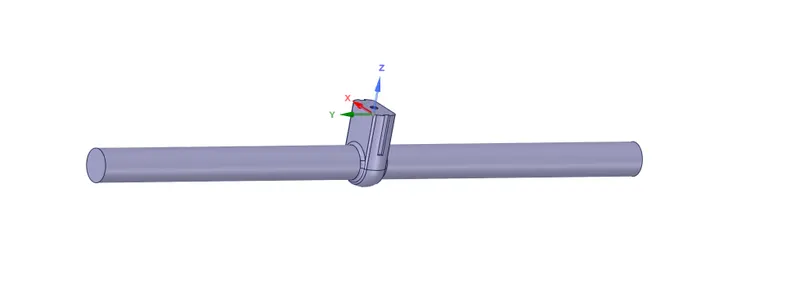
a. Gate valve:

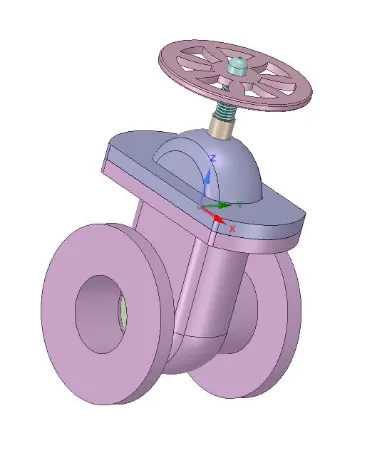
b. Extending the geometry of the pipe by using the pull tool:

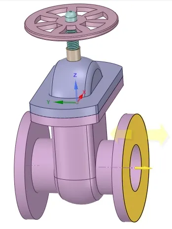
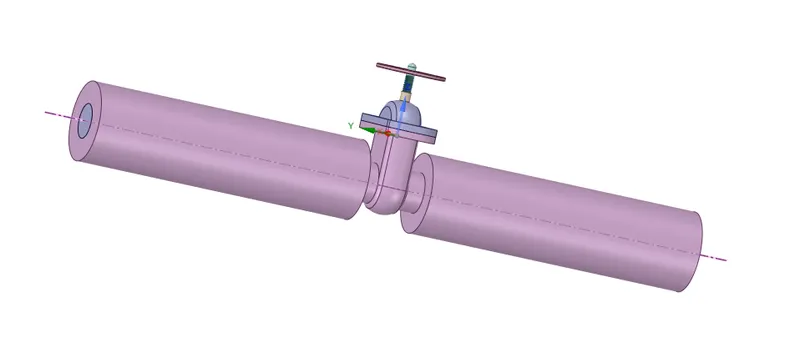
c. Moving the gate disc upward accordingly and to perform parametric study based on the movement on the gate disc

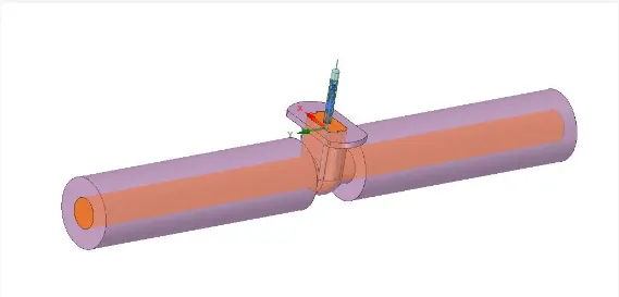
d. Performing volume extract to get the fluid volume so that the fluid analysis can be performed.

e. Viewing the change in gate disc by inserting section plane,

Meshing:

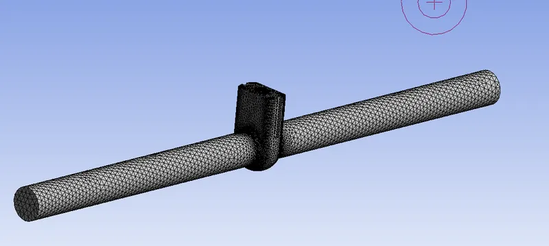
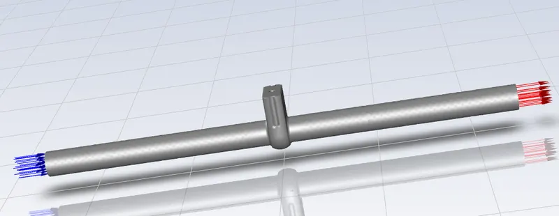
Name the inlet and outlet by face selecting command

Elemental size:92.82mm

no. of elements: 137317

3.Fluent set up:

General setup:

Physics set up:

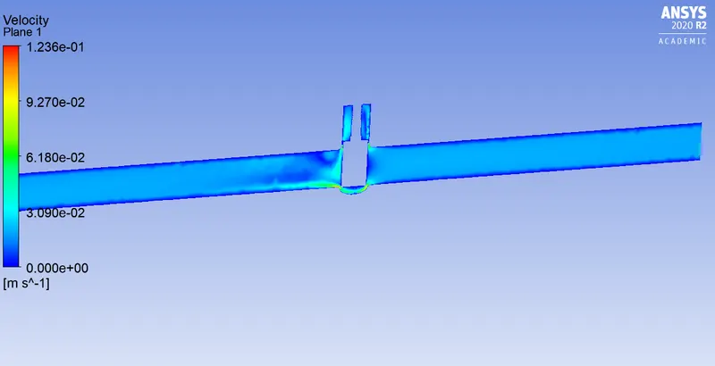
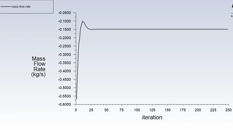
Case 1:10mm lift of gate

Residual plot:

velocity contour:

Mass flow rate:

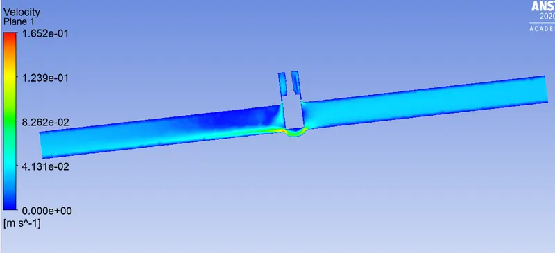
Case 1:20mm lift of gate

Residual plot:

velocity contour:

Mass flow rate:

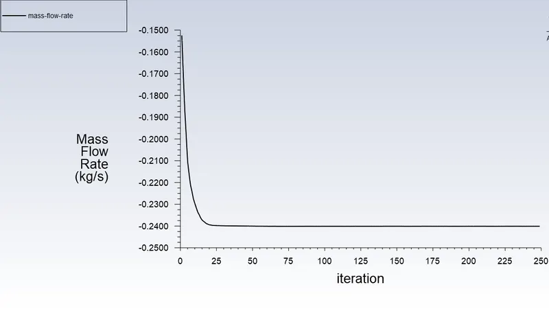
Case 1:35mm lift of gate

Residual plot: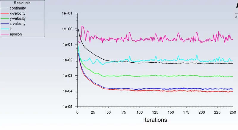

velocity contour: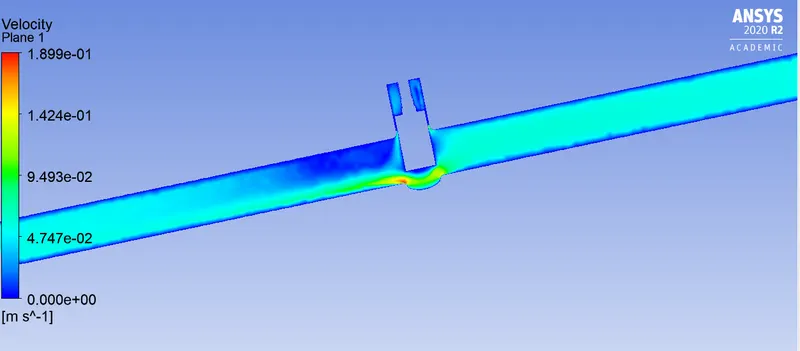

Mass flow rate: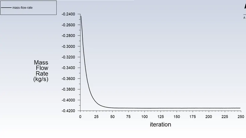

Case 1:45mm lift of gate

Residual plot:

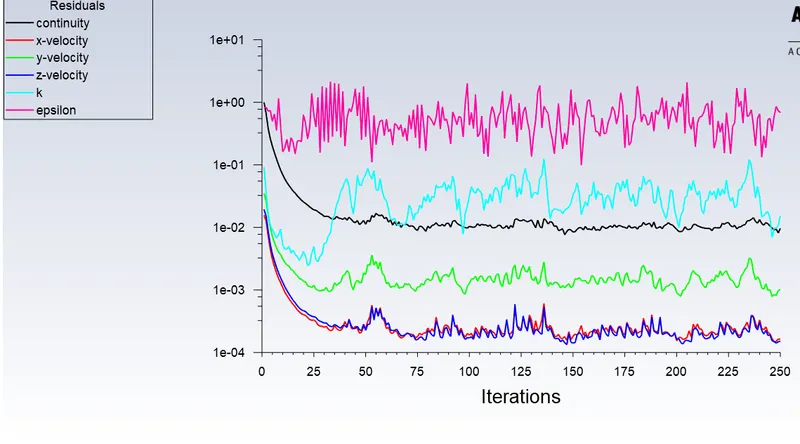
velocity contour: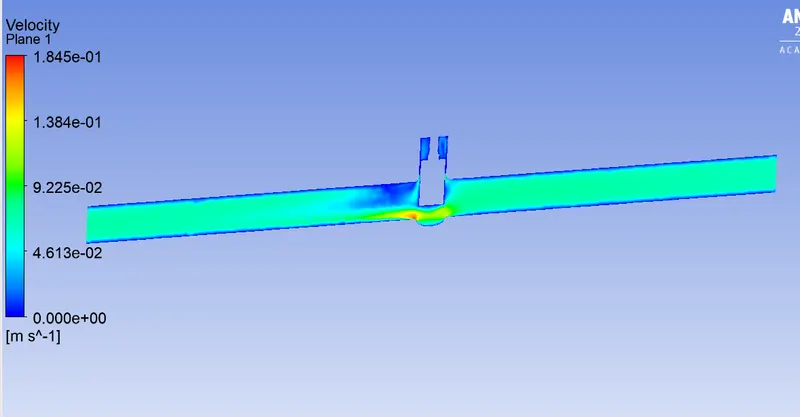

Mass flow rate: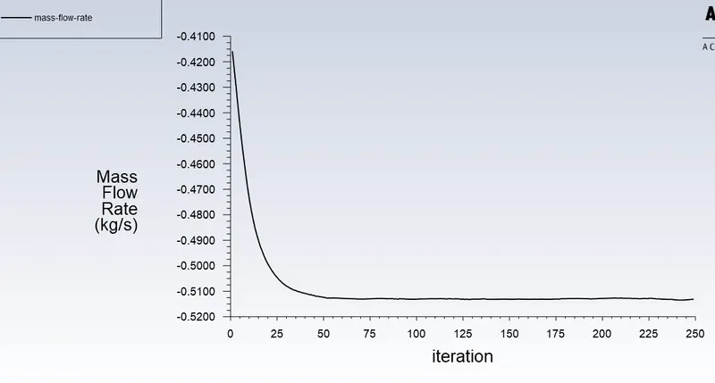

Case 1:50mm lift of gate

Residual plot: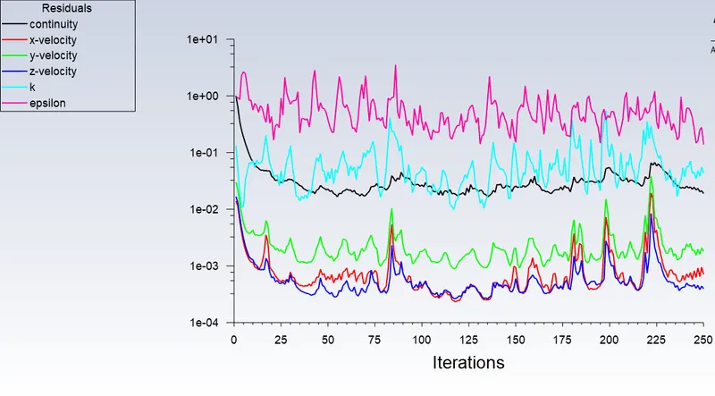

velocity contour: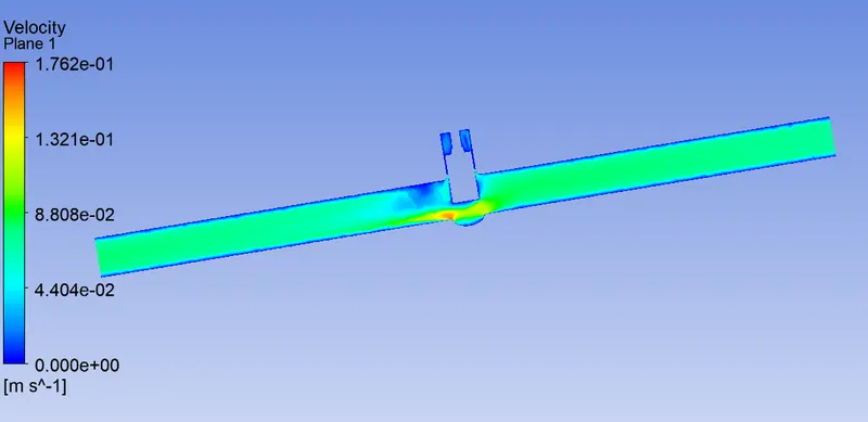

Mass flow rate: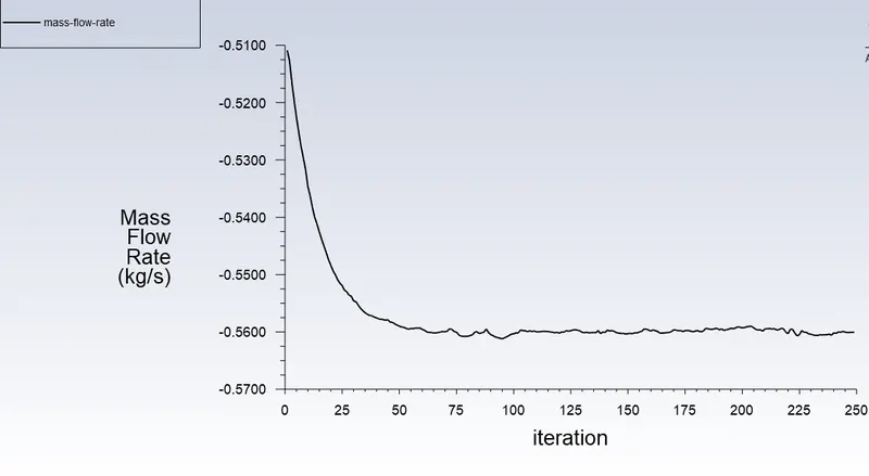

Case 1:60mm lift of gate

Residual plot: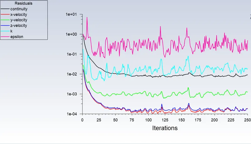

velocity contour: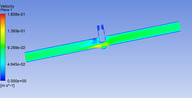

Mass flow rate:

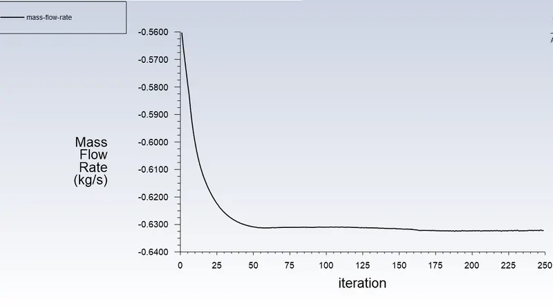
Case 1:80mm lift of gate

Residual plot: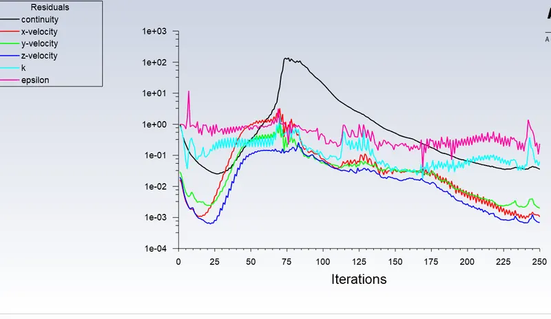

velocity contour: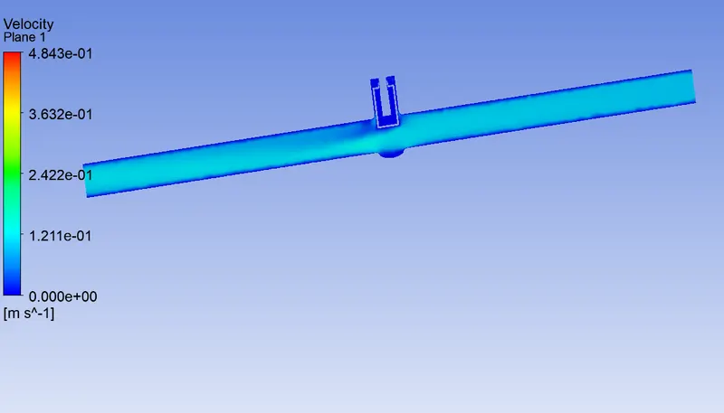

Mass flow rate:

parametric study table:

Calculation of flow coefficient and flow factor :

According to SI units, they can be converted to,

Here, Q=1kg/s i.e. Q=3.6 m^3/hr

ΔP= 10pascal

= 10 * 10^-5 bar (pascal to bar conversion= 1*10^-5 bar)

ΔP= 10^-4 bar.

Also, 1 ÷ √(10^-4) = 100

K_v = Q * (( Mass flow rate value in each case) * 1 /√(10^-4))

Lift	mass flow rate in `kgs^-1`	Q (`m^3(hr)^-1`	flow factor	flow coefficient
10	0.1490	0.5364	53.64	62.01
20	0.24008	0.8642	86.42	99.9
35	0.415	1.494	149.4	172.71
45	0.5131	1.847	184.7	213.52
50	0.559	2.012	201.2	232.60
60	0.632	2.275	227.5	263.0
80	0.7637	2.533	253.3	292.83

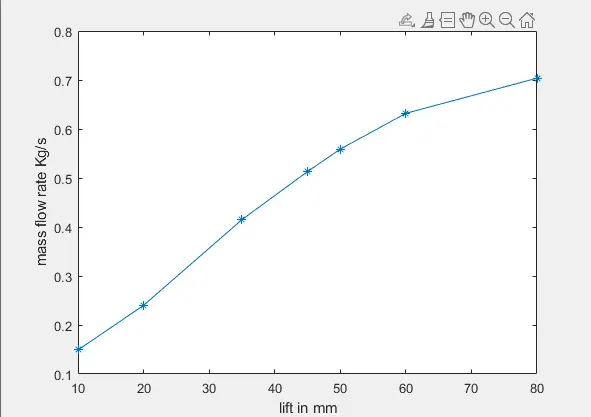
Lift v/s mass flow rate graph

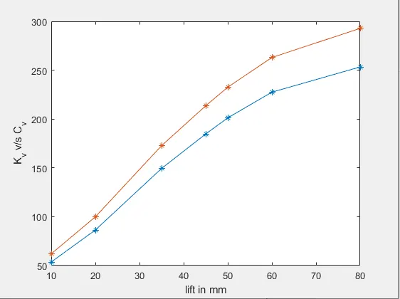
the flow coefficient and flow factor for each lift plot:

Conclusion:

From the plot, it can be concluded that as the gate disc rises, mass flow rate, flow coefficient and flow factor increases gradually.

1. From the above contours, as the opening of the gate disc increases-the mass flow rate of fluid also increases.
2. It is observed that the maximum lift of the gate disk helps the fluid flow freely without any disturbance or restriction in the flow.
3. Similarly, from the generated data it is noted that for different valve openings there is a rise in the flow coefficient.
4. Hence, all the parameters studied above are directly proportional i.e. as lift increases the flow factor and the flow coefficient raises.
5. The calculated flow coefficient is useful to find the overall efficiency of the gate valve.
6. The velocity contour shows how the fluid flow behaves on opening the gate valve and also indicates the maximum velocity throughout the flow.

The parametric study on the gate valve is performed by varying the lift from 10% to 80%. During the parametric study several parameters and its effects are plotted for representation. It's clear that the fluid flow rate gradually increases with the increase in the lift of the gate disc. Also the flow coefficient and the flow factors are plotted in order to observe the effect during the simulation. Hence in this study the effect of opening the gate valve on the fluid characteristics are established.