Week 6 - CHT Analysis on a Graphics card

AIM:

To study and perform a steady-state conjugate heat transfer analysis on a graphics card model.

OBJECTIVE:

• Run the simulation by varying the velocity from 1m/sec to 5m/sec for at least 3 velocities.
• Find out the maximum temperature and heat transfer coefficient attained by the processor.
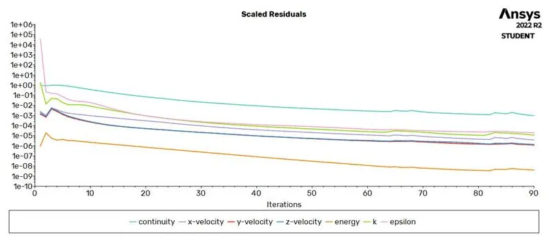
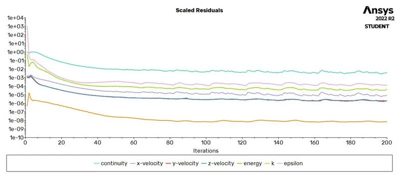
• Prove that the simulation has achieved convergence with appropriate images and plots.
• Identify potential hotspots on the model.

GRAPHICS CARD:

The Graphics card is the expansion card that generates a feed of output images on a computer monitor. The Graphics card(GPU) is one of the main components used in PCs for additional processing, reducing the load on the central processing units(CPUs).

For the higher-performing tasks heat generated by the processor is much high which is bad for the circuit board. Hence we use FINS to dissipate heat from the processor. This indeed helps the GPU to perform a given task for a longer duration because of proper heat dissipation by the fins.

FINS

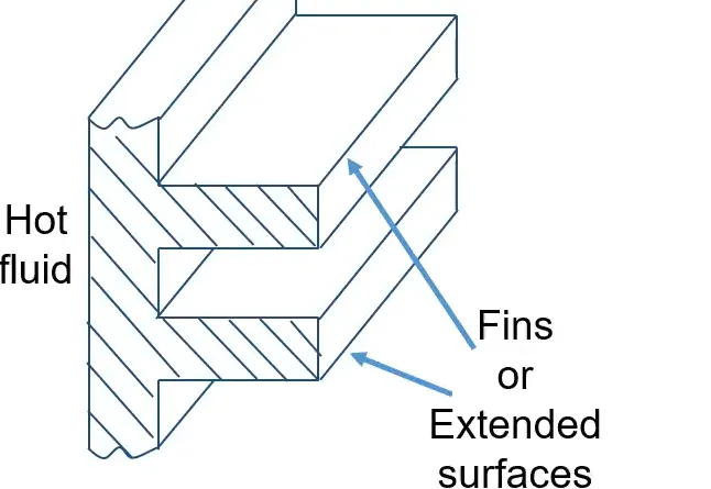
Fins are extended surfaces attached to the primary object to be cooled. Heat conducts from the primary objects to the fins. The fin surface provides an extra surface for heat dissipation to take place via convection. It is a conduction-convection system employed to dissipate heat from the surface at a faster rate to the surrounding fluids. There are different types of fins such as rectangular, circular, Pin fin, conical, etc. Here in the graphic card, we are using rectangular fins.

THEORY OF CONJUGATE HEAT TRANSFER

Conjugate heat transfer corresponds with the combination of heat transfer in solids and heat transfer in fluids. In solids, conduction often dominates whereas, in fluids, convection usually dominates. Conjugate heat transfer is observed in many situations. The exchange of thermal energy between the two physical bodies is called a study of Heat Transfer, the rate of transferred heat is directly proportional to the temperature difference between the bodies.

modes of heat transfer

1. Conduction: diffusion of heat due to temperature gradients. A measure of the amount of conduction for a given gradient is heat conductivity.
2. Convection: when heat is carried away by moving fluid. The flow can either be caused by external influences, forced convection; or by buoyancy forces, natural convection.

DETAILED PROCEDURE FOR SIMULATING GRAPHIC CARD USING ANSYS FLUENT SOFTWARE

In ANSYS fluent we have three major steps to solve CFD problems Pre-processing, Solver, and Post-processing.

• Pre-processing involves cleaning up the models and generating the mesh here its geometry, mesh.
• Solver involves setting up the problem statements such as solver used, boundary conditions, methods, report definitions, etc here the solver used in Ansys is setup.
• Post-processing involves obtaining the simulated contours, graphs, and animations here in Ansys it is Results.

GEOMETRY

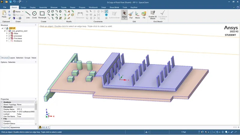
• Initially, I am importing the GRAPHIC CARD (.STEP) file into the space claim.
• Sharing the topology by using the share tool which is available in the workbench(Share topology is done for information exchanges between the adjacent surfaces or in order to have common node points between solid and external volume surfaces). Hence under the WORKBENCH=> select the SHARE option.

MESH

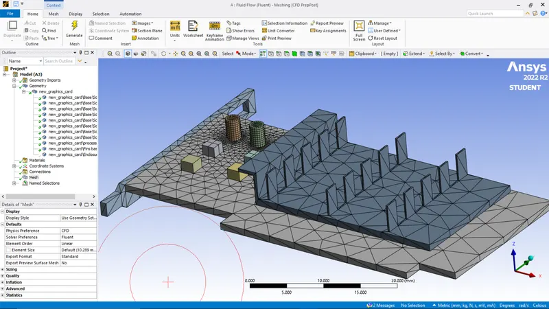
• For meshing, I have taken the element size of 10mm. By doing this we can observe that the graphic mesh is not fine enough to capture the model as shown below.

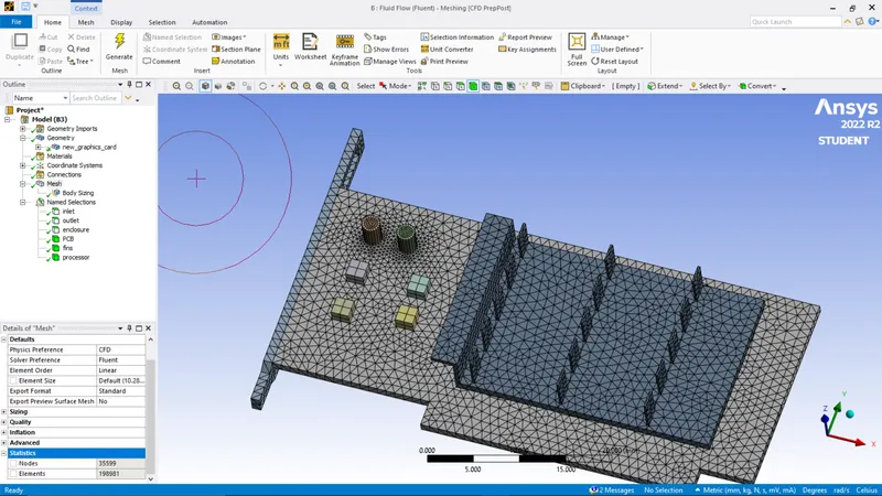
• Hence in order to capture the geometry, We can insert the body sizing under this we have to enable the capture curvature(To capture the geometry to get refined mesh) finally by giving the mesh element size as 1mm. Instead of going to mesh update, we have cleared the generated mesh the give update the mesh. We can see refined mesh as shown below.

SETUP AND SOLUTIONS

• In this, we provide fundamental physics, types of solver, boundary conditions, and type of turbulent model used.
• Initially, we go for the SOLVER option here we are the type of solver used is PRESSURE BASED SOLVER (M<0.3), and since the variable is not varying with respect to time select the STEADY STATE option.
• In the following step for the PHYSICS, the window selects the VISCOUS option we get the window opened up. Here we are selecting the type of viscous model which is a TURBULENT model (k-epsilon). Since we have to calculate the temperature energy is turned on.
• Here for solids materials aluminum, silicon, and polystyrene this assigned under the solids sections there are properties are stated below.

ALUMINUM thermal conductivity(k=202.4 W/mK) specific heat capacity(cp=871 J/kg K) density(rho=2719 kg/m3)

SILICON thermal conductivity(k=153 W/mK) specific heat capacity(cp=703 J/kg K) density(rho=2330 kg/m3)

POLYSTYRENE thermal conductivity(k=0.027 W/mK) specific heat capacity(cp=1210 J/kg K) density(rho=55 kg/m3)

• For fins, I am assigning an aluminum, a processor as silicon, and PCB as polystyrene.
• In cell zone conditions we change from fluids to solid structures for respective parts such as fins, processor, and PCB. For heat generation under the processor, I give the heat source term as 2Watt divided by the volume of the processor.
• We are giving the BOUNDARY conditions for the inlet velocity as 1m/s, 3m/s, 5m/s, and the default temperature as 300K.
• The hybrid method is used for initialization.
• Run this simulation based on solution convergence hence here this simulation converges at 200 iterations.
• Finally, we are obtaining the graph heat transfer coefficient for the processor, temperature of the processor, and contour plots.

RESULTS

• Then for obtaining the contour plot for variation of temperature and velocity, Under PLANE we do a COLOR option to change the VARIABLE option.

SIMULATION FOR COARSE MESH OF 1mm WITH FORCED CONVECTION OF 1m/s

The average heat transfer coefficient of the processor is 4.8704 W/m2 K.

The average temperature of the processor is 358.51 K.

SIMULATION FOR FINNER MESH OF 1mm WITH FORCED CONVECTION OF 1m/s

Scaled residual plot

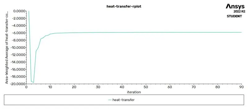
Averaged heat transfer coefficient plot

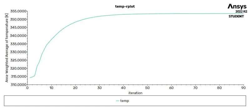
Averaged heat temperature plot

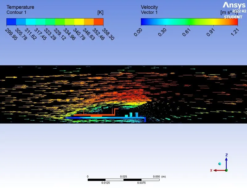
CONTOUR PLOT OF VELOCITY AND TEMPERATURE

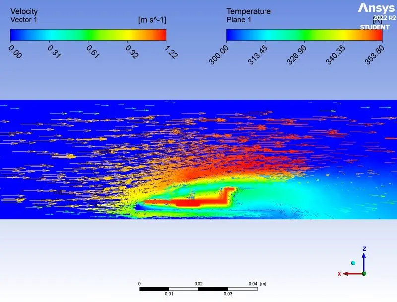
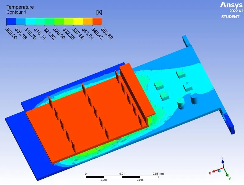
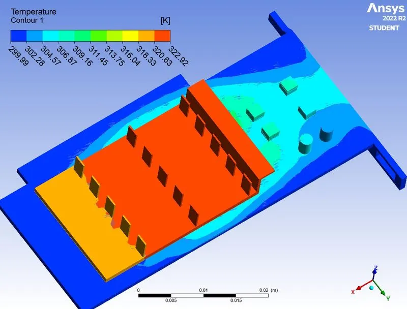
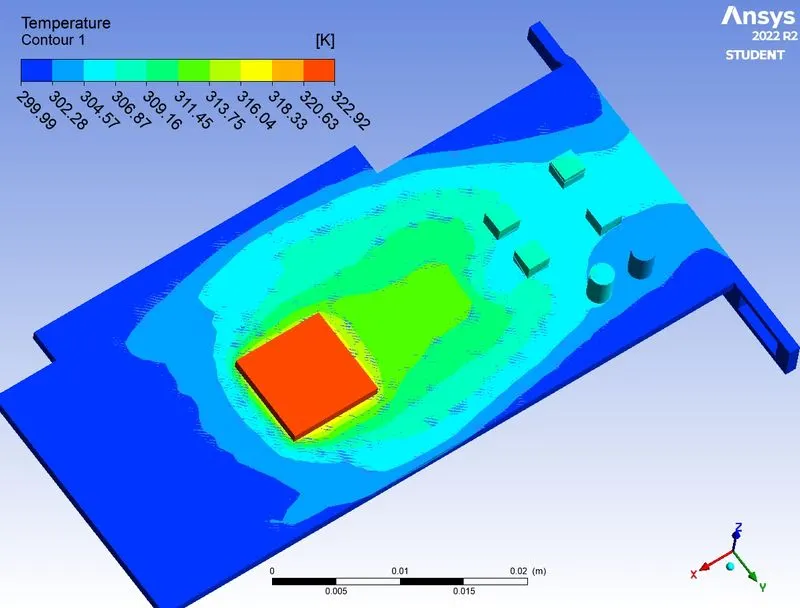
TEMPERATURE HOTSPOTS

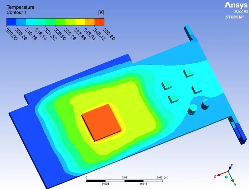
The average heat transfer coefficient of the processor is 5.8504 W/m2 K.

The average temperature of the processor is 353.51 K.

SIMULATION FOR FINNER MESH OF 1mm WITH FORCED CONVECTION OF 3m/s

Scaled residual plot

Averaged heat transfer coefficient plot

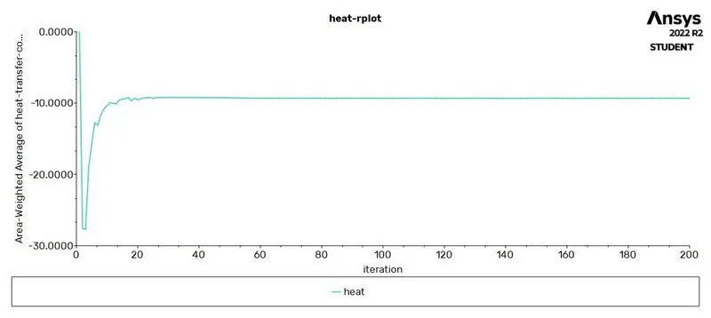
Averaged heat temperature plot

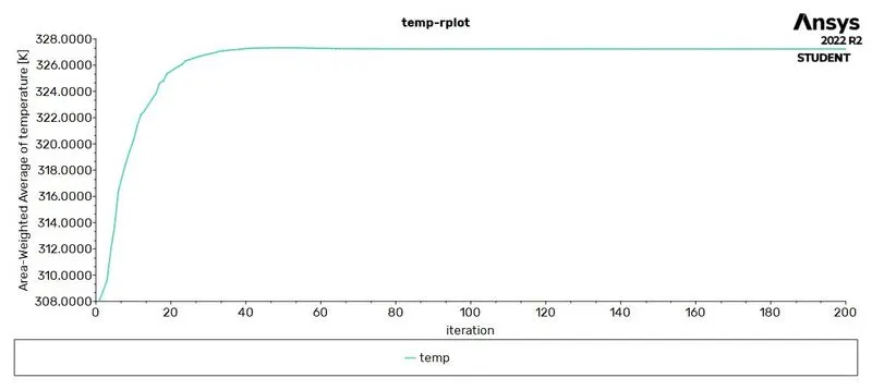
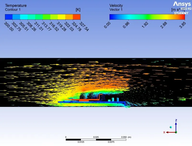
CONTOUR PLOT OF VELOCITY AND TEMPERATURE

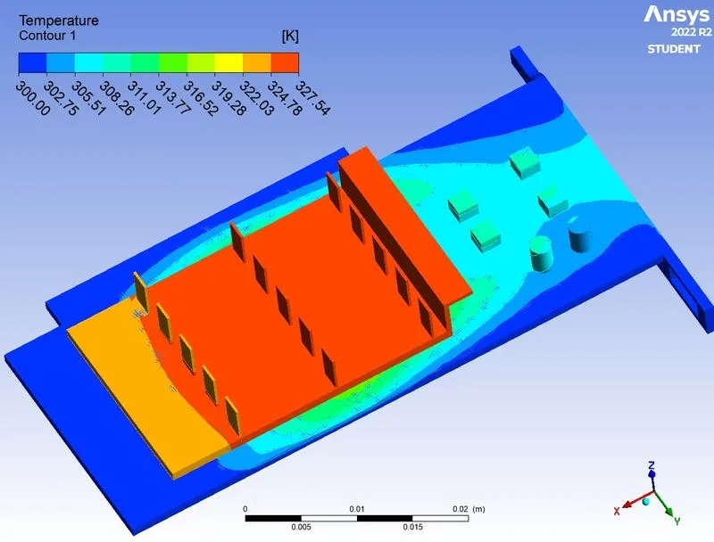
TEMPERATURE HOTSPOTS

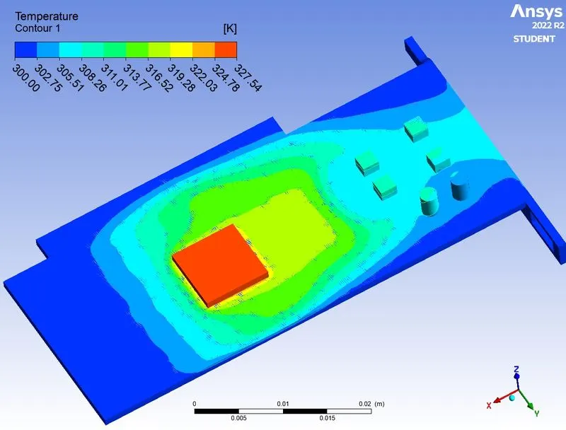
The average heat transfer coefficient of the processor is 9.366 W/m2 K.

The average temperature of the processor is 327.51 K.

SIMULATION FOR FINNER MESH OF 1mm WITH FORCED CONVECTION OF 5m/s

Scaled residual plot

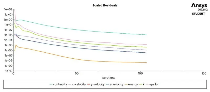
Averaged heat transfer coefficient plot

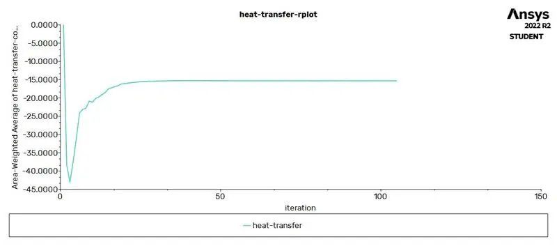
Averaged heat temperature plot

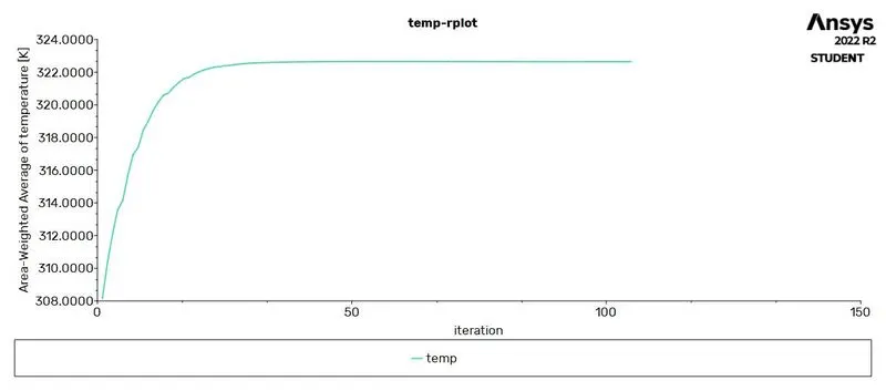
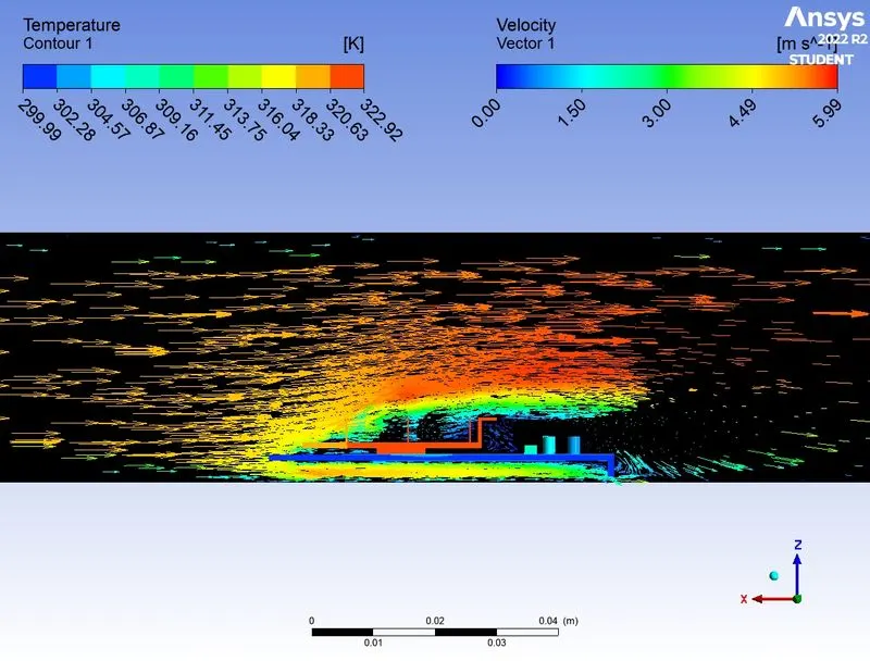
CONTOUR PLOT OF VELOCITY AND TEMPERATURE

TEMPERATURE HOTSPOTS

The average heat transfer coefficient of the processor is 15.317 W/m2 K.

The average temperature of the processor is 322.64 K.

CONCLUSIONS

• Finner the mesh on the graphics greater the physics can be captured such as temperature and velocity.
• By varying the velocity from 1 to 5 we can see that force convection increases the heat transfer coefficient of the processor and greater the heat dissipation from the fins. This can be observed based on the temperature contour plots.