Week 9 - Parametric study on Gate valve.

AIM:

To study and perform a parametric study on the gate valve simulation by using the ANSYS fluent software.

OBJECTIVE:

• Perform a parametric study on the gate valve simulation by setting the opening from 10 % to 80%.
• Obtain the mass flow rates at the outlet for each design point.
• Calculate the flow coefficient and flow factor for each opening and plot the graph.
• Discussing the results of the mass flow rate and flow coefficient.

GATE VALVE

Gate valves are mainly used in industries to shut the flow of fluid rather than the flow regulation. They can be found in petrochemical industries, power plants, and widely in the pipeline industries. Here we are performing the analysis for the wedge gate valve.

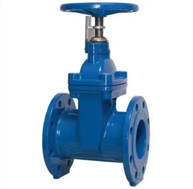
Gate valves work by inserting a rectangular gate or wedge into the path of a flowing fluid. They are operated by a threaded stem that connects the actuator (generally a hand wheel or motor) to the stem of the gate. If the valve has a rising stem its position can be seen just by looking at the position of the stem. A gate valve is used to control the fluid flow by lifting and descending the gate. A gate distinct feature is to provide an unobstructed passageway, which includes minimal pressure loss over the valve.

When the gate is fully opened there is no restriction to the flow hence the pressure drop is low comparatively. Generally, the gate valve are fully closed or fully open as the partially opened valves may experience vibration which may lead to excessive wear. A gate valve's main component is the body, seat, gate, stem, bonnet, and actuator. the primary mechanism is straight forward where the handwheel is rotated to move the gate up and down via threads. they require more than a 360-degree turn to fully open the valve.

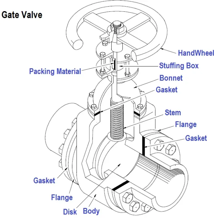
Gate valves tend to be slightly cheaper than ball valves of the same size and quality. They are slower in actuation than quarter-turn valves and are for applications where valve operation is infrequent, such as isolating valves. Gate valves should be used either fully open or fully closed, not to regulate flow. Automated gate valves exist with either an electric or pneumatic actuator, but a manual gate valve is cost-effective since they have infrequent usage. Gate valves are widely used for all types of applications and are suitable for both above-ground and underground installation. They are suitable for most fluids including steam, water, oil, gas, etc.

DETAILED PROCEDURE FOR PERFORMING PARAMETRIC STUDY FOR GATE VALVE USING ANSYS FLUENT

PARAMETRIZING THE LIFT

For the parametric study, the input parameter that needs to be parametrized is the lift of the gate disc. For this use the move feature and select the gate-disc body and move along the Z direction. Then enter the value beside which is P button can be seen and click the same. Now the fluid region needs to get updated for the change in geometry which can be done by the update of the volume body in the context option.

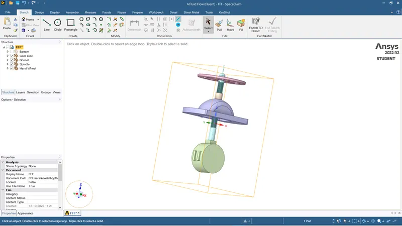
The solid geometry consists of the bottom housing, handwheel, spindle, bonnet, and gate valve. The fluid moves from the inlet to the outlet, and the gate valve is used to restrict this motion, and this is actuated manually by turning the handwheel which is supported by the bonnet and is connected via the spindle. When a lesser mass flow is required at the outlet, the gate valve is lowered, which restricts the mass flow of the fluid at the outlet. The mass flow rate of the fluid at the outlet varies with the lift of the gate valve stopper, and that is to be simulated.

GEOMETRY using SpaceClaim

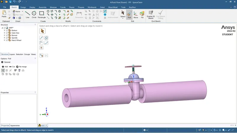
• In order to study the flow we have to extend both surfaces using the pull option for 800mm on both sides.
• To simulate the effect of the stopper on the mass flow rate of the fluid at the outlet the stopper is moved 10mm in the positive Z-direction so that the flow path is partially open. This is parametrized.

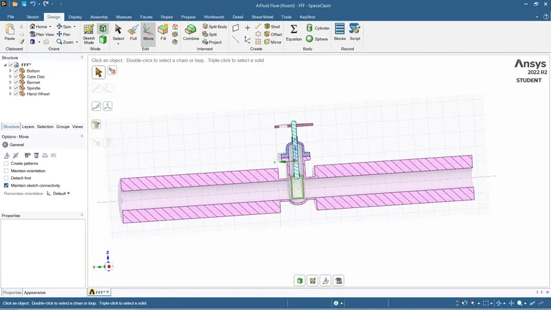
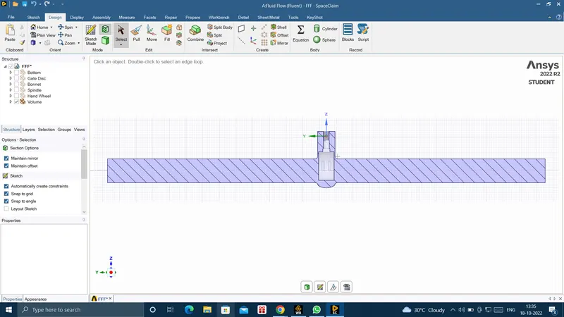
• Next, the fluid is extracted from the solid geometry. The parameterization helps us change its value and compute the required output parameters without having to repeat the same processes again. Since we are not interested in the analysis of solid geometry, it is suppressed.

MESH

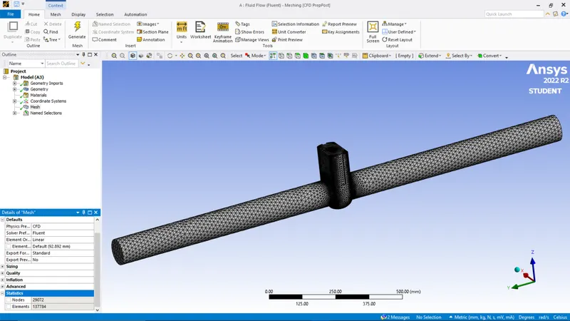
• I am using sizing mesh option=> insert=>sizing methods(give respective mesh size) similarly internal enclosure, Also I am using sizing mesh option=> insert=>sizing methods(give respective mesh size).
• Here I am inserting the size for the wedge surface as 5mm.
• Respective name selection is done for inlet and outlet conditions.
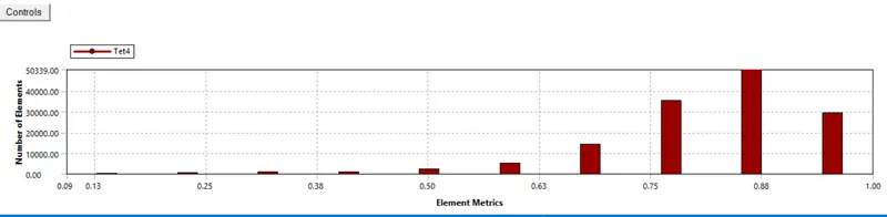
• Finally, the mesh element size for the entire geometry is given as 92mm(check for the quality of the mesh).

SETUP AND SOLUTION

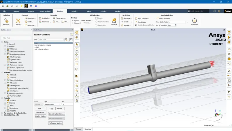
• In this, we provide fundamental physics, types of solver, boundary conditions, and type of turbulent model used.
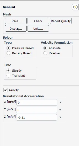
• Initially, we go for the SOLVER option here we are the type of solver used is PRESSURE BASED SOLVER (M<0.3), and since the variable is not varying with respect to time select the STEADY STATE option. Also, we provide acceleration due to gravity(g=-9.81 in the Z direction).

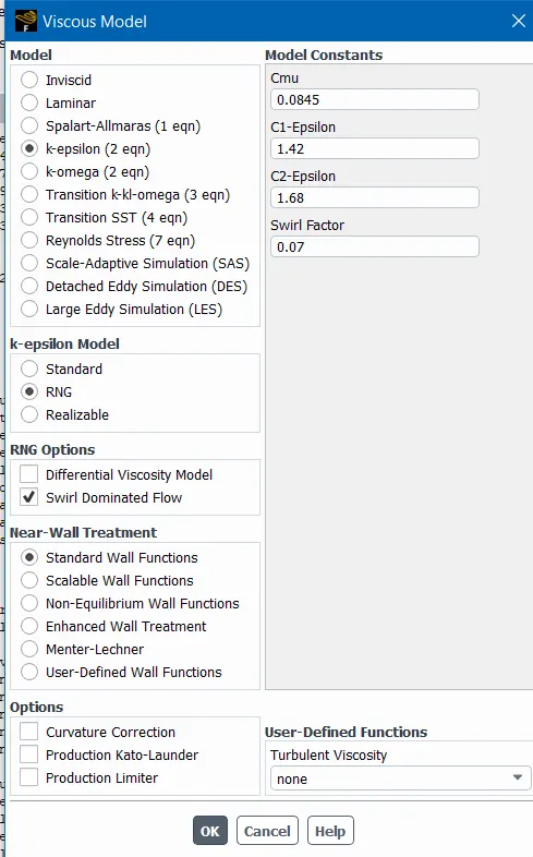
• In the following step for the PHYSICS, the window selects the VISCOUS option we get the window opened up. Here we are selecting the type of viscous model which is a TURBULENT model (k-epsilon) and RNG with the swirl-dominated flow, we are using the standard wall functions option(for capturing better physics).

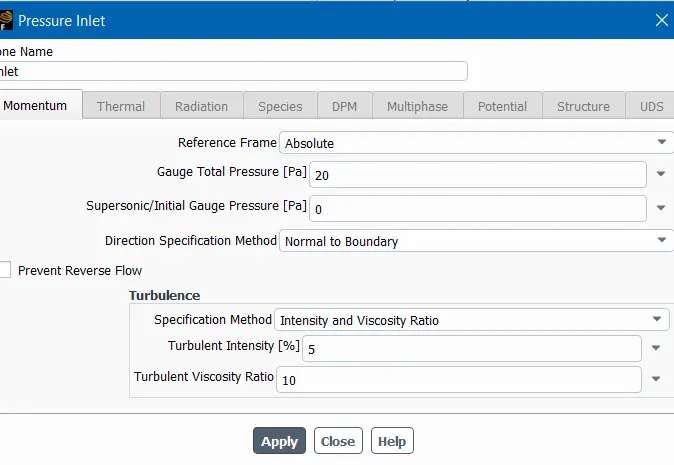
• We are giving the BOUNDARY conditions for the inlet pressure as 20Pa.

• Change the fluid from air to water, and provide the mass flow rate graph for the outlet to study the mass flow rate.
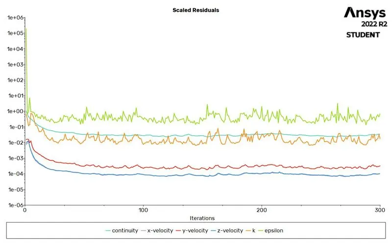
• Finally do hybrid initialization and run for the 300 iterations to check for convergence.

RESULTS

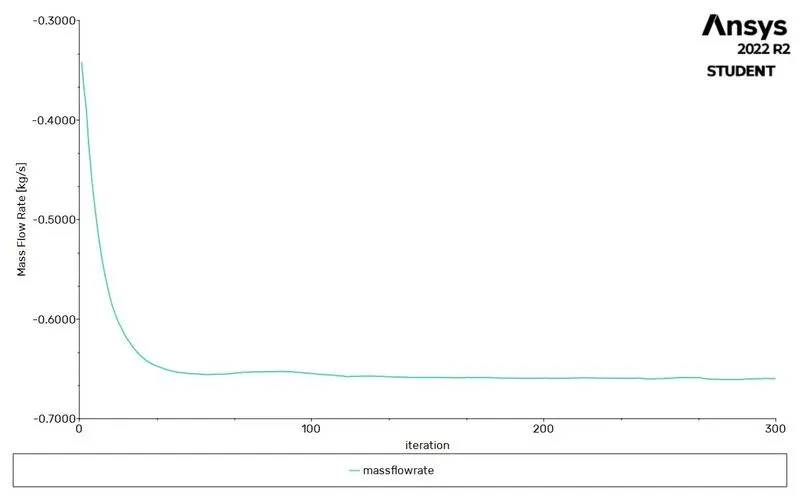
A flux report of the mass flow rate is created and it is defined as an output parameter so as to calculate this property at different positions of the wedge. The plot below gives the mass flow rate of the fluid at the outlet at a 10mm lift of the wedge.

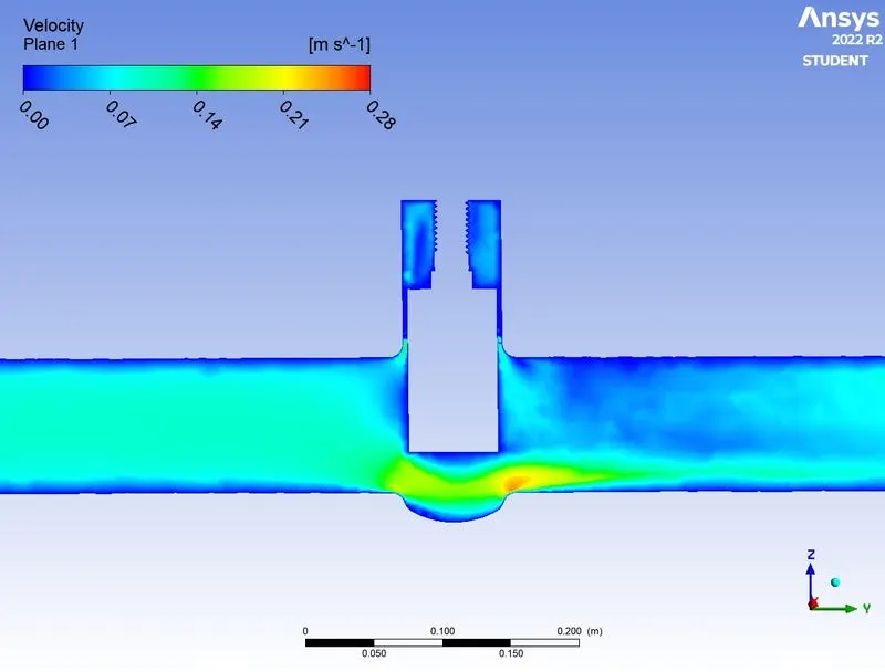
For 3 cases results are shown

CASE 1: For 20mm

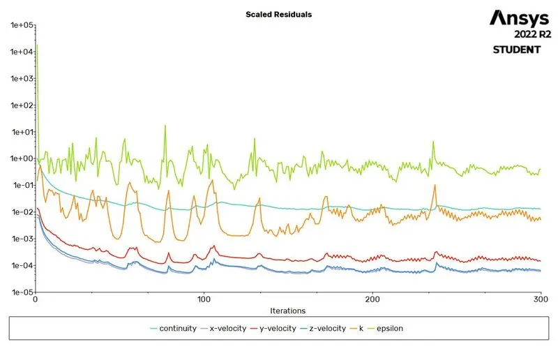
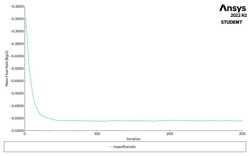
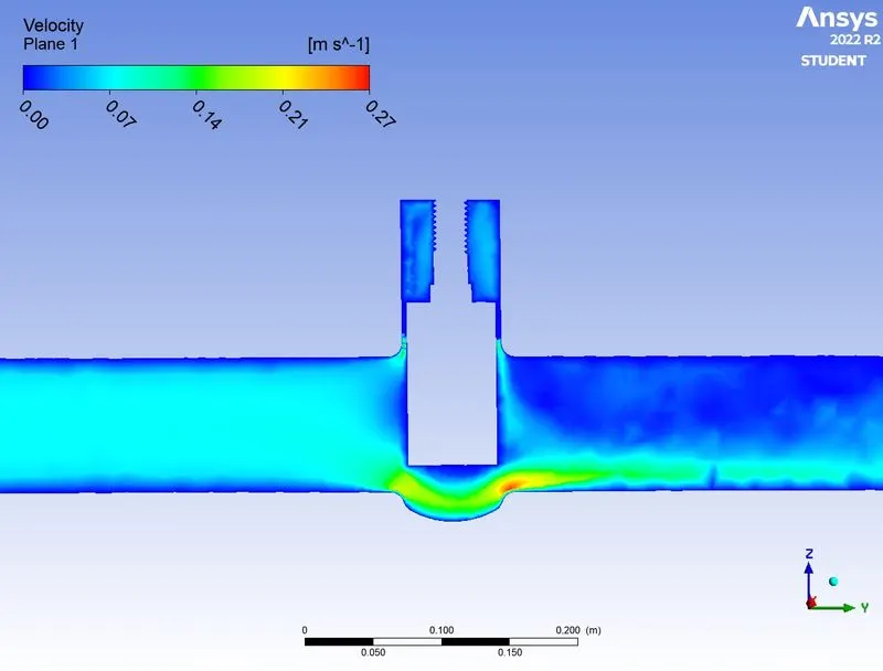
CASE 2: For 30mm

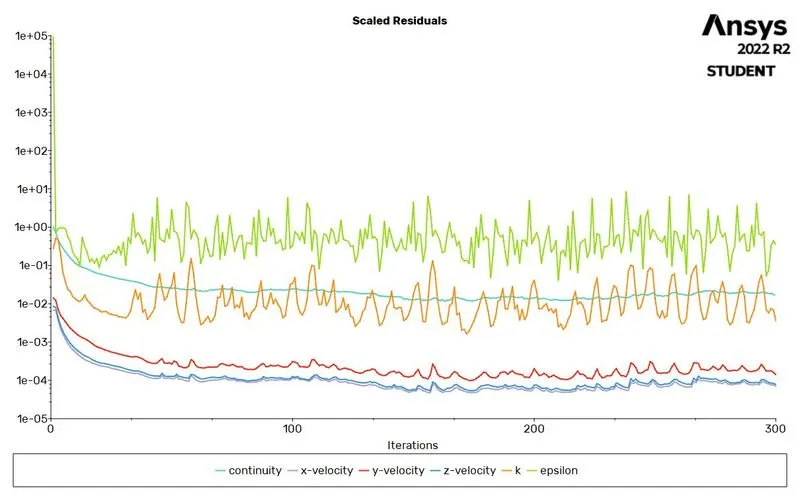
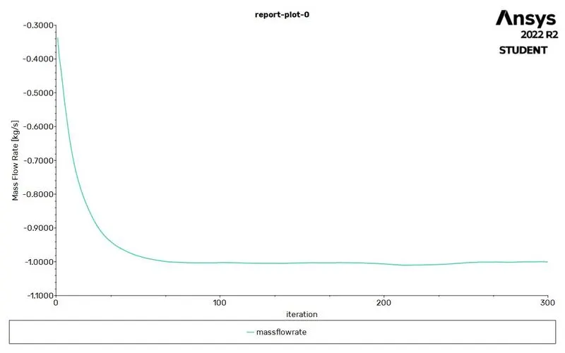
CASE 3: For 60mm

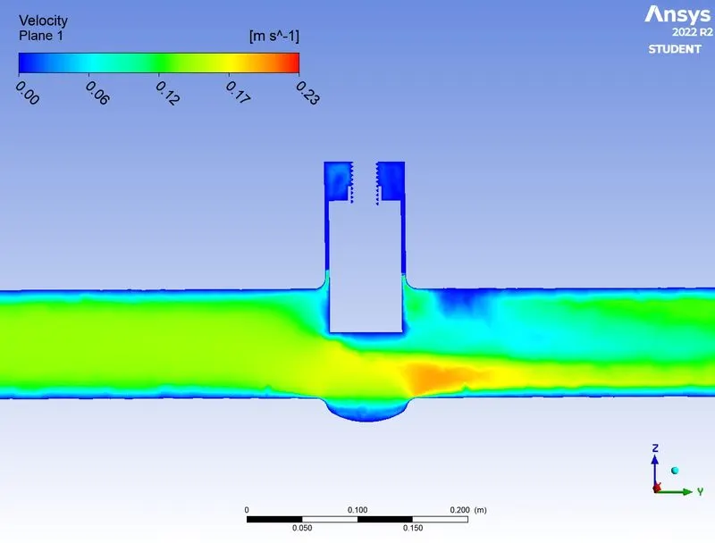
Next, we move on to the parameters tab to calculate the mass flow rates for the different wedge heights, and the following results were obtained

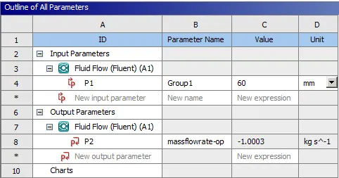
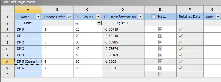
The negative signs for the mass flow rates imply that the fluid is exiting the domain. The mass flow rate is calculated for the stopper lifts from 10mm to 70mm. The mass flow rate increases with the increase in the lift of the stopper. When the stopper is lifted gradually, the space available for the passage of the fluid increases hence the mass flow increases. When we perform the parametric study, Ansys automatically changes the mesh as per new geometry using the same mesh specifications given earlier, and solves and calculates the output parameters, thereby saving time comparatively if it was done manually.

NUMERICAL CALCULATIONS FOR FLOW COEFFICIENT AND FLOW FACTOR

The flow coefficient(Cv) of a device is a relative measure of its efficiency in allowing fluid flow. It describes the relationship between the pressure drop across an orifice valve or other assembly and the corresponding flow rate.

`Cv=Q*sqrt((SG)/(triangleP))`

where:

Q is the rate of flow (expressed in US gallons per minute)

SG is the specific gravity of the fluid (SG for water= 1)

ΔP is the pressure drop across the valve (expressed in psi).

The metric equivalent flow factor(Kv) is calculated using metric units

`Kv=Q*sqrt((SG)/(triangleP)`

where:

Q is the rate of flow (expressed in m^3/h)

SG is the specific gravity of the fluid (SG for water= 1)

∆P is the pressure drop across the valve (expressed in a bar).

Kv can be calculated from Cv using the equation:

`Kv=0.865*Cv`

The following table gives the flow factor and flow coefficient of the fluid at different valve displacement magnitudes. Before the parameters are substituted into the formula, the units must be converted to the specific units

Inlet pressure is considered as P=20pa

magnitude of valve displacement	Mass flow rate(Kg/s)	Pressure outlet(Pa)	Flow factor(Kv)	Flow coefficient(Cv)
10	0.33718	0.9710	101.886	88.131
20	0.50418	2.1851	195.506	169.112
30	0.65985	3.7567	215.399	186.32
40	0.78674	5.3669	270.6862	234.14
50	0.90169	6.9154	328.1331	283.83
60	1.0003	8.4864	388.086	335.69
70	1.1051	10.3764	468.9662	405.62

TREND OF FLOW AND FACTOR COEFFICIENTS WITH THE PERCENTAGE OF VALVE OPEN

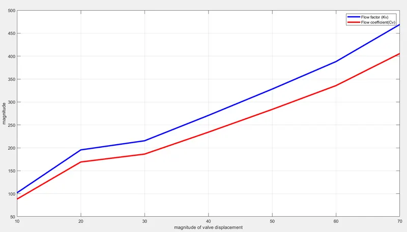
From the above trend plots, we can say that with the increase in the opening of the gate valve the mass flow rate also increases. Along with the mass flow rate, the flow coefficient and flow factor also increase.

CONCLUSIONS:

• Parametric studies allow you to nominate parameters for evaluation, define the parameter range, specify the design constraints, and analyze the results of each parameter variation. When you have the configurations generated you can then evaluate your simulation. You can further refine the parameters or design constraints until satisfied with the results.

• Once you determine that a configuration satisfies your design needs, you are able to promote that configuration back to the model as a CAD edit. You are prompted to make changes. Using the parametric study method saves a lot of time in the simulations which require performing the same operations for different settings multiple times.

• In the parametric study of the gate valve, it was found that as the valve wedge is lifted gradually, the mass flow rate of the fluid, and hence the flow factor and flow coefficient increases.