Week 5 - Rayleigh Taylor Instability

AIM:-

1. What are some practical CFD models that have been based on the mathematical analysis of Rayleigh Taylor waves? In your own words, explain how these mathematical models have been adapted for CFD calculations.
2. Perform the Rayleigh Taylor instability simulation for 2 different mesh sizes with the base mesh being 0.5 mm. Compare the results by showing the animations( Attach them from your google drive). Observe the differences in the animation and explain the effect of mesh size on simulation. Also, explain why a steady-state approach might not be suitable for these types of simulation.[ Choose Air and Water for this simulation]
3. Run one more simulation with water and user-defined material(density = 400 kg/m³, viscosity = 0.001 kg/m-s) for refined mesh.
4. Define the Atwood Number. Find out the Atwood number for both the cases and explain how the variation in Atwood number in the above two cases affects the behavior of the instability.

CONTENTS

Chapter 1 - Definition of Rayleigh Taylor Model.

Chapter 2 - Definition of Multiphase flow modelling and itS Modelling Methods.

Chapter 3 - Detailed Explaination of Volume Of Fluid model.

Chapter 4 - Mathematics - Governing Equations involved in Volume of Fluid.

Chapter 5 - Practical CFD Models that are based on mathematical analysis of Rayleigh Taylor Waves and How are they implemented.

Chapter 6 - Problem setup and Simulation.

1. Case 1 - Simulating with Base mesh = 0.5 mm.

2. Case 2 - Simulating with some more Dense mesh.

3. Why Steady State simulation is not prefered for these types of simulations.

4. Case 3 - Simlating with water and User Defined Material, With Given Values of density and Viscosity for refined mesh.

Chapter 7 - Detailed Explaination of Atwood Number and its variation of above simulated results.

Chapter 8 - Conclusion. and Why Transient simulation is used in this case.

CHAPTER 1

DEFINITION OF RAYLEIGH TAYLOR MODEL

Rayleigh Taylor Model -

The Rayleigh–Taylor instability, or RT instability, is an Instability of an Interface between two Fluids of different densities which occurs when the lighter fluid is pushing the heavier fluid.

Source - Wikipedia

Examples - Behavior of water suspended above oil in the gravity of earth.

CHAPTER 2

DEFINITION OF MULTIPHASE FLOW MODELLING AND ITS Modelling Methods

Multiphase Flow Modelling

A multiphase flow is defined as one in which more than one phase (i.e., gas, solid and liquid) occurs. Such flows are ubiquitous in industry, examples being gas-liquid flows in evaporators and condensers, gas-liquid-solid flows in chemical reactors, solid-gas flows in pneumatic conveying, etc.

In multiphase flows, solid phases are denoted by the subscript S, liquid phases by the subscript L and gas phases by the subscript G.

Some of the main characteristics of these three types of phases are as follows:

Multi-phase flow consist of two major phases:

1. Particle (dispersed) phase,
2. Continuous (Eulerian) phase

1. Particle (Dispersed) phase

• This phase consists of bubbles, particles, or drops, and the continuous phase as the fluid in which these particles are generally immersed.
• The particles can be composed of solid, liquid, or gas.

2. Continuous (Eulerian) Phase

• It is based on the Eulerian hypothesis of continuous phase
• The continuous fluid can be a liquid or a gas

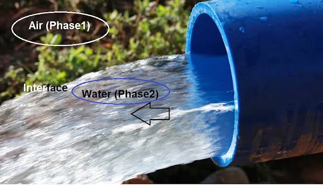
Source Google - Explaining the Multiphase Flow via picture

INTERFACE

• Due to difference in chemical or physical structures, a narrow region between phases is observed as demarcation. This is called an interface
• To distinguish two adjacent phases or matters, a mathematical function for the interface is generally used for numerical (CFD) modeling.

Modelling Methods.

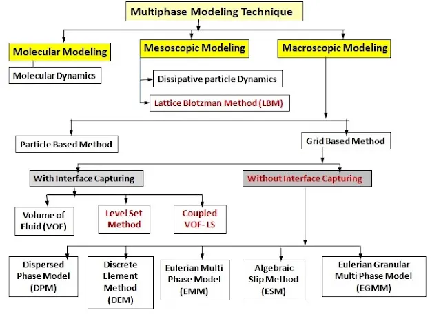
(NOTE - Here we are using VOF (Volume of Fluid ) Method with interface modelled in geometry modelling using spaceclaim)

CHAPTER 3

DETAILED EXPLAINATION OF VOLUME OF FLUID MODEL

In this method, the different phases are modeled mathematically considering as interpenetrating continua. For a given volume, a particular phase cannot be occupied by the other phases. Hence, the concept of volume fraction is introduced to define the phases. Total sum of volume fraction is 1

Interface Capturing Method

• This approach is used for a fixed Eulerian mesh.
• It is designed for two or more immiscible fluids where the position of the interface between the fluids is necessary.
• A mathematical function is used at the interface to discriminate two adjacent phases.
• The volume of fluid (VOF) method is mass conservative but interface is not sharp (diffusive) and surface tension is not correctly accounted.

In the VOF method the indicator function α takes value 1 in one phase and 0 in the other. We have a continuity equation :

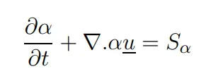
The velocity u comes from solving the NSE for the mixture

The indicator function

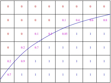
• represents the position of the interface and is advected by the flow, Computationally the interface smeared over 3-4 cells.
• 4 schemes in Fluent – geometric, donor/acceptor, Euler explicit and implicit.

Characteristics of VOF

Characteristic Features	Volume Of Fluid (VOF)
Advection Equation	`(delvarphi)/(delt) + ui (delvarphi)/(delx) = 0`
Physical Interpration	Transport Equation of Mass Fraction (concentration)
Location of Interface	Usually at 0.5
Re Processing of Interface	Reconstruction of free surfaces (SLIC, PLIC)
Accuracy of interface	Diffusive Interface
Mass Conservative at interface	Yes

CHAPTER 4

MATHEMATICAL MODELLING (GOVERNING EQUATION) OF VOLUME OF FLUID MODEL

• The method is based on the idea of a so-called fraction function . It is a scalar function, defined as the integral of a fluid's Characteristic Function in the Control Volume namely the volume of a computational grid cell.
• The volume fraction of each fluid is tracked through every cell in the computational grid, while all fluids share a single set of momentum equations, i.e. one for each spatial direction.
• From a cell-volume averaged perspective, when a cell is empty of the tracked phase, the value of is zero;
• when the cell is full of tracked phase,;
• when the cell contains an interface between the tracked and non-tracked volumes, .
• From a perspective of a local point that contains no volume, is a discontinuous function insofar as its value jumps from 0 to 1 when the local point moves from the non-tracked to the tracked phase.
• The normal direction of the fluid interface is found where the value of changes most rapidly.
• With this method, the free-surface is not defined sharply, instead it is distributed over the height of a cell.
• Thus, in order to attain accurate results, local grid refinements have to be done.
• The refinement criterion is simple, cells with have to be refined.
• A method for this, known as the marker and micro-cell method,

Continuity Equation.

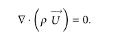
Taking into accout of Gravity Momentum Equation is defined as

Energy Equation.

The different methods for treating VOF can be roughly divided into three categories, namely

• the donor-acceptor formulation,
• higher order differencing schemes and
• line techniques.

CHAPTER 5

Practical CFD Models that are based on mathematical analysis of Rayleigh Taylor Waves and How are they implemented.

CFD models that have been based on the mathematical analysis of Rayleigh Taylor waves.

1. Mass diffusion model:

• The mass diffusion equation describes the transport of mass and energy due to model viscosity and hence drives actual mixing in the fluids.Even if any configuration is Rayleigh-Taylor unstable, the diffusion process could be responsible for significsnt mixing if the viscosity is sufficiently large.

2. Single fluid model:

a. Potential flow model:

• The model is valid for all instabillity changes from the linear stage through the early non-linear to the asymptotic but limited to Atwood number = 1. In this model, single-mode peturbation expands the flow equations to second-order around the bubble tips, hence obtaining an ordinary differential equation for the bubble velocity.

b. Buoyancy drag model:

• It is valid for every Atwood number but limited to the non-linear stages of the instability. It uses ordinary differential equations to evolve the width of the mixing layer. The bubble, or spike, amplitudes are discribed by balancing the interia, buoyancy and drag forces.
• These models cannot model multiple mixing interfaces; cannot be easily extended to 2 or 3 dimensions, and as a rule, do not adress demixing, also known as counter gradient transport

c. Besnard-Harlow-Rauenzahn(BHR)

• It is a more advanced version of the single fluid model. The BHR model is based upon the evolution equations arising from second-order correlations and gradient-diffusion approximations. Using a mass-weighted averaged decomposition, the original BHR model includes full transport equations for the Reynold stresses, turbulent mass-flux velocity, density fluctuation and the turbulent kinetic energy dissipation rate.

3 Multi Fluid model:

• These models use a separate set of equations for each fluid in addition to the main flow equations and provide an accurate modeling framework for demixing by correctly capturing the relative motion of the different fluid fragments.
• The first step for the development of turbulence models is to perform Reynold averaging of the governing equations and resultant terms.

a. Two equation K-L turbulence model:

• The K-L turbulence model involves equations for turbulent kinematic energy K and turbulent length scale L. The starting point for deriving the model equations are the buoyancy-drag models for the self-similar growth of RT instabilities.

b. Three equation K-L-a turbulence model:

• The three equation model was developed as an extension to the two-equation K-L model by including a third equation for the turbulent mass-flux velocity.

c. Four equation K-L-a-b turbulence model:

• The four equation model was developed as an extension to the three-equation K-L model by including a fourth equation for density specific volume covariance. The model can accurately reflect the effects of the changes in the density fluctuations.

1. Kelvin - Helmholtz
2. Richtmyer–Meshkov instability (RMI)
3. Plateau–Rayleigh instability

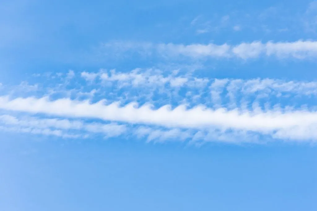
Kelvin-Helmholtz (KH)

instability typically occurs between two immiscible fluids with a velocity difference across their interface. This instability can be observed, for example, as a natural phenomenon of certain cloud patterns. These patterns are characterized by the generation of small-scale motion at the interface, which later leads to the formation of an unstable interfacial vortex street. This generates spiral structures at the fluid-fluid interface. Wave formation on still water due to blowing wind is another common example of this instability.

Richtmyer–Meshkov instability (RMI)

• Occurs when two fluids of different density are impulsively accelerated.
• Normally this is by the passage of a Shock wave.
• The development of the instability begins with small amplitude perturbations which initially grow linearly with time.
• This is followed by a nonlinear regime with bubbles appearing in the case of a light fluid penetrating a heavy fluid, and with spikes appearing in the case of a heavy fluid penetrating a light fluid.
• A chaotic regime eventually is reached and the two fluids mix.
• This instability can be considered the impulsive-acceleration limit of the Rayleigh Taylor Instability

Example

1. During the implosion of an inertial Confinment fusion target, the hot shell material surrounding the cold fuel layer is shock-accelerated. This instability is also seen in magnetised Target fusion. Mixing of the shell material and fuel is not desired and efforts are made to minimize any tiny imperfections or irregularities which will be magnified by RMI.

2. Supersonic combustion in a Scramjet may benefit from RMI as the fuel-oxidants interface is enhanced by the breakup of the fuel into finer droplets.

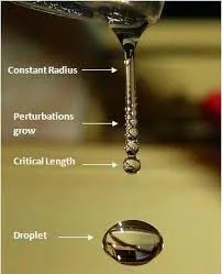
Plateau–Rayleigh instability,

• often just called the Rayleigh instability, explains why and how a falling stream of fluid breaks up into smaller packets with the same volume but less surface area.
• It is part of a greater branch of fluid dynamics concerned with fluid - thread Breakup

Examples

1.Water Dripping from Tap

A special case of this is the formation of small droplets when water is dripping from a faucet/tap. When a segment of water begins to separate from the faucet, a neck is formed and then stretched. If the diameter of the faucet is big enough, the neck doesn't get sucked back in, and it undergoes a Plateau–Rayleigh instability and collapses into a small droplet.

2. Male Urination

Another everyday example of Plateau–Rayleigh instability occurs in urination, particularly standing male urination. The stream of urine experiences instability after about 15 cm (6 inches), breaking into droplets, which causes significant splash-back on impacting a surface. By contrast, if the stream contacts a surface while still in a stable state – such as by urinating directly against a urinal or wall – splash-back is almost completely eliminated.

3. Inkjet Printing

Continuous ink jet printers (as opposed to drop-on-demand ink jet printers) generate a cylindrical stream of ink that breaks up into droplets prior to staining printer paper. By adjusting the size of the droplets using tunable temperature or pressure perturbations and imparting electrical charge to the ink, inkjet printers then steer the stream of droplets using electrostatics to form specific patterns on printer paper

CHAPTER 6

PROBLEM SETUP AND SIMULATION

https://www.youtube.com/channel/UCxPFvEioszvvKo5QPYaC5wA

The following simplifying assumptions are taken into account: 

• Flows and transfers in the two phases are laminar and incompressible 
• The effect of the superficial tension is negligible 
• The liquid and gas flows are two dimensional and transient 

CASE 1

Simulation Using Base mesh (0.5 mm)

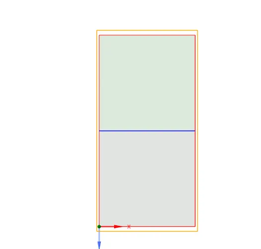
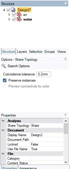
Step 1 :- Geometry Creation

• Create two rectangles one upon another
• Convert sketching into surface by using pull method
• Enable the share option as it creates the interface between two surfaces

1st section contains Water

2nd Section contains Air

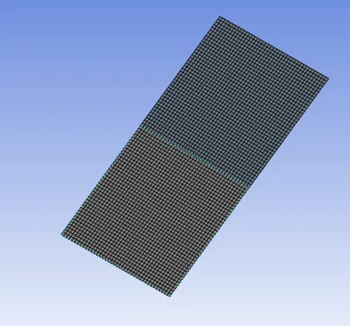
Step 2 - Mesh Cretion

• Just a base line mesh with 0.5 mm is created using Mesh Option

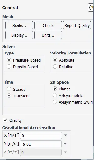
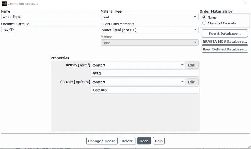
Step 3 - Setup the Physics

1. Import the mesh file into Fluent
2. In General Tab make sure it is transient based solver
3. Enable Gravity
4. check the Quality of mesh
5. Enable the Viscous model ----> Laminar
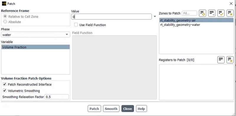
6. Enable the multiphase flow -----> VOF ------>Set to Implicit
7. Choose Primary Phase and Secondary Phase
8. Initialise ----> Standard Initialisation
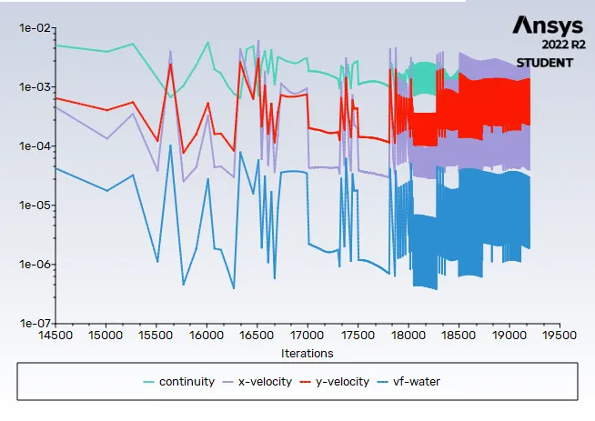
9. Set Courant Number as 0.2
10. Patch Water as 1 and air as 0
11. Add Contours of Velocity of Water

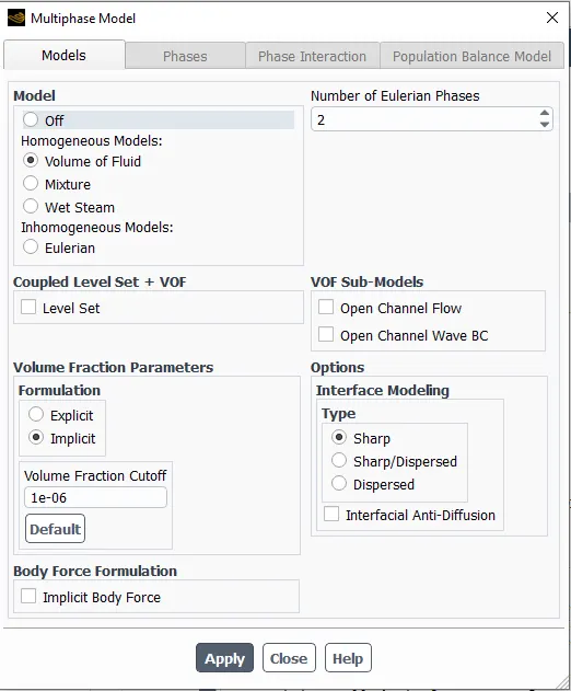
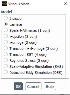
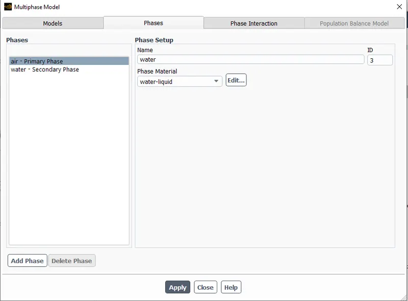
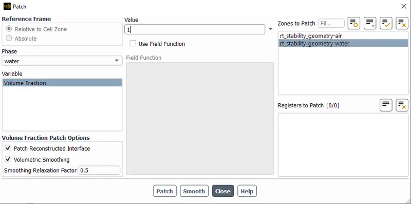
Step 4 - Post Processing and Results Viewing.

Video

CASE 2

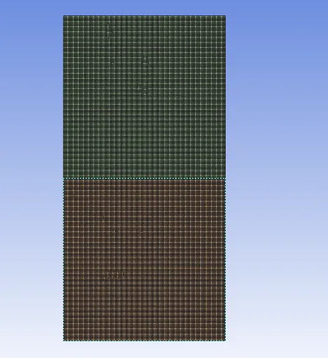
Mesh Size 0.2mm

Follow step 1

MESH SETUP

Remaining follow same steps

CASE 3

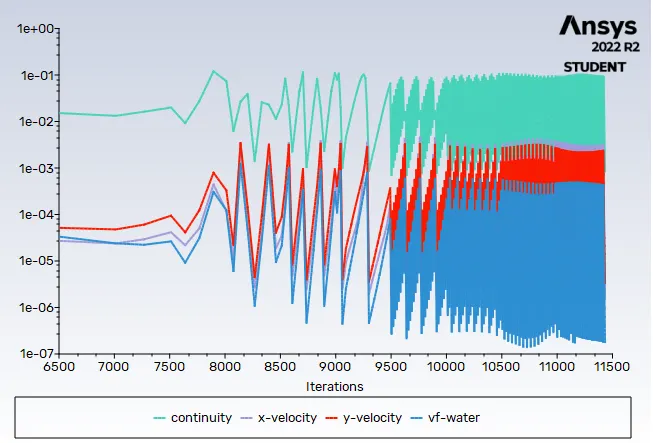
User defined material with density 400 kg/m3 and Viscosity 0.001

Steps same as above withe same finer mesh

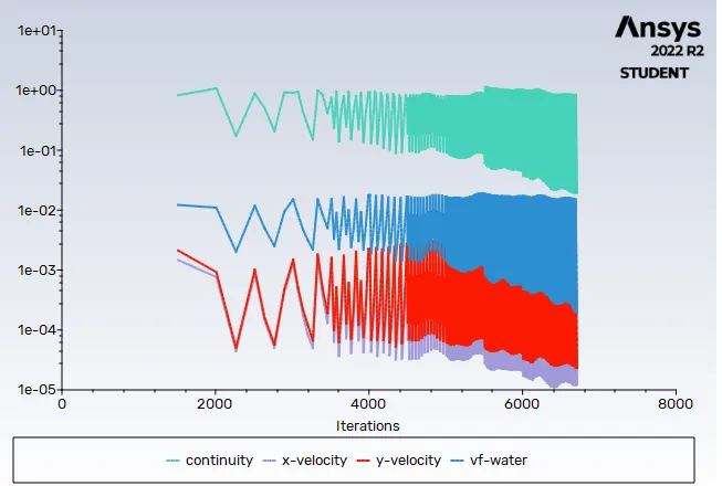
CHAPTER 7

Detailed Explaination of Atwood Number and its variation of above simulated results.

• The Atwood number is a dimensionless number in fluid dynamics used in the study of hydrodynamic instabilities in density stratified flows.
• It is a dimensionless density ratio related to the density of heavier fluid and the density of lighter fluid. (The difference in the fluid densities divided by their sum).
• Atwood number is an important parameter in the study of Rayleigh–Taylor instability.
• For Atwood number close to 0, RT instability flows take the form of symmetric “fingers” of fluid;
• for Atwood number close to 1, the much lighter fluid “below” the heavier fluid takes the form of larger bubble-like plumes.

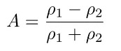
A	Atwood number (dimensionless)
ρ1	Density of heavier fluid (kg/m3)
ρ2	Density of lighter fluid. (kg/m3)

So Considering above Cases we can calculate the atwood number by using the above formula

So using the above formula we get Atwood NUmber as

Case 1 and Case 2 = 0.99754

Case 3 = 0.4285

Chapter 8 -

Conclusion.

Here we talk why

SO we can conclude that

• Higher the atwood Number the Instabilites are sudden and Reach steady state more rapidly
• Lower the Atwood Number Instabilites Take time and Reach steady state slowly
• From the animation video it is able to visualize the RT instability of two fluid accurately. It is also concluded that fine meshing provide a clear picture of simulation as compared to baselinemeshing.

RTI evolves in three distinct stages:

• Linear stability,
• mushroom head(falling) or bubble(rising) formation,
• long term evolution due to bubble merging and mixing.

For low Atwood number, bubble and mushroom head shape is relatively symmetrical, the disturbances or perturbations are linear for a larger time.

for large Atwood number, bubble and mushroom head shape is less symmetrical, also it occurs very rapidly at an accelerating rate which leads to a nonlinear growth rate.

• Since the simulation involves capturing instabilities that are changing in an unpredictable manner as a function of time, the transient approach is preferred over the steady-state approach.