Rayleigh Taylor Instability

Aim: Perform Rayleigh Taylor instability simulation

Objectives:

• Perform simulation for 2 different mesh sizes.
• Compare the results by showing the animation
• Explain the effect of mesh size on simulation
• Explain reason why a steady state approach is not suitable
• Run simulation with water and user defined material
• Find Atwood number for the cases

Theory:

Rayleigh Taylor Instability:

The Rayleigh–Taylor instability, or RT instability (after Lord Rayleigh and G. I. Taylor), is an instability of an interface between two fluids of different densities which occurs when the lighter fluid is pushing the heavier fluid.

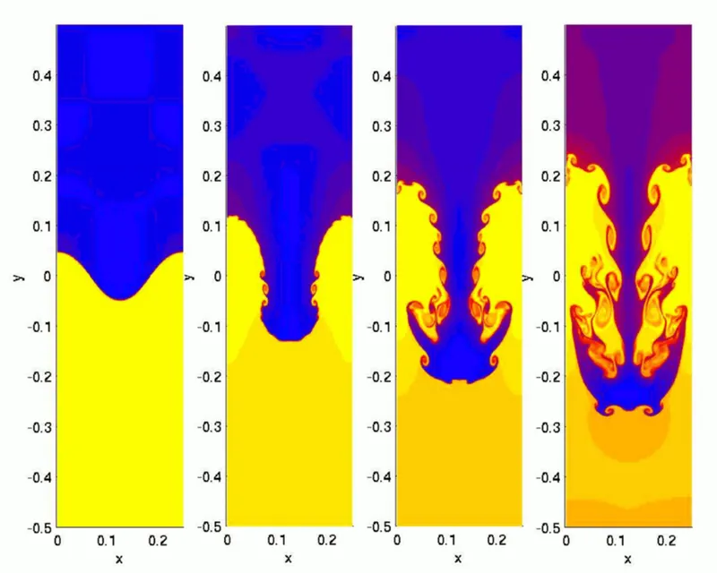
Examples:

• behaviour of water suspended above oil in the gravity of Earth
• mushroom clouds like those from volcanic eruptions and atmospheric nuclear explosions,
• supernova explosions in which expanding core gas is accelerated into denser shell gas,
• instabilities in plasma fusion reactors and inertial confinement fusion.

Steps in Rayleigh Taylor instability:

The evolution of the RTI follows four main stages.

1. The perturbation amplitudes are small when compared to their wavelengths, the equations of motion can be linearized, resulting in exponential instability growth. In the early portion of this stage, a sinusoidal initial perturbation retains its sinusoidal shape. However, after the end of this first stage, when non-linear effects begin to appear, one observes the beginnings of the formation of the ubiquitous mushroom-shaped spikes (fluid structures of heavy fluid growing into light fluid) and bubbles (fluid structures of light fluid growing into heavy fluid).
2. The growth of the mushroom structures continues in the second stage and can be modelled using buoyancy drag models, resulting in a growth rate that is approximately constant in time. At this point, nonlinear terms in the equations of motion can no longer be ignored.
3. The spikes and bubbles then begin to interact with one another in the third stage. Bubble merging takes place, where the nonlinear interaction of mode coupling acts to combine smaller spikes and bubbles to produce larger ones. Also, bubble competition takes places, where spikes and bubbles of smaller wavelength that have become saturated are enveloped by larger ones that have not yet saturated.
4. This eventually develops into a region of turbulent mixing, which is the fourth and final stage in the evolution. It is generally assumed that the mixing region that finally develops is self-similar and turbulent, provided that the Reynolds number is sufficiently large.

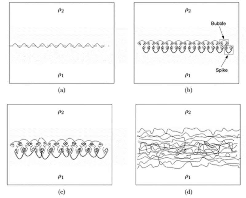
This figure represents the evolution of the Rayleigh–Taylor instability from small wavelength perturbations at the interface (a) which grow into the ubiquitous mushroom shaped spikes (fluid structures of heavy into light fluid) and bubbles (fluid structures of light into heavy fluid) (b) and these fluid structures interact due to bubble merging and competition (c) eventually developing into a mixing region (d). Here ρ2 represents the heavy fluid and ρ1 represents the light fluid. Gravity is acting downward and the system is RT unstable.

Practical CFD example of Rayleigh-Taylor instability:

Water-oil example of Rayleigh-Taylor instability:

Water suspended atop oil is an everyday example of Rayleigh–Taylor instability, and it may be modelled by two completely plane-parallel layers of immiscible fluid, the denser fluid on top of the less dense one and both subject to the Earth's gravity. The equilibrium here is unstable to any perturbations or disturbances of the interface: if a parcel of heavier fluid is displaced downward with an equal volume of lighter fluid displaced upwards, the potential energy of the configuration is lower than the initial state. Thus the disturbance will grow and lead to a further release of potential energy, as the denser material moves down under the (effective) gravitational field, and the less dense material is further displaced upwards.

As the RT instability develops, the initial perturbations progress from a linear growth phase into a non-linear growth phase, eventually developing "plumes" flowing upwards (in the gravitational buoyancy sense) and "spikes" falling downwards. In the linear phase, the fluid movement can be closely approximated by linear equations, and the amplitude of perturbations is growing exponentially with time. In the non-linear phase, perturbation amplitude is too large for a linear approximation, and non-linear equations are required to describe fluid motions. In general, the density disparity between the fluids determines the structure of the subsequent non-linear RT instability flows.

Rayleigh-Taylor CFD simulation of water-air multiphase :

Base Case setup:

1.Geometry:

• Create a rectangle of 20 by 20 mm in space claim, use pull tool to create a new component name it as air

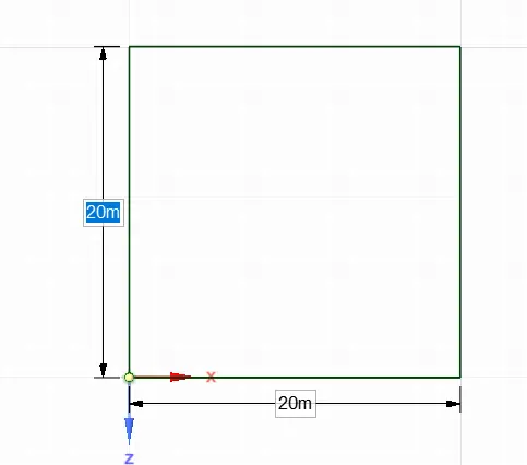
• similarly create another 20 by 20 mm rectangle above the air component we have just created, use pull tool and create another component and name it as water

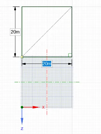
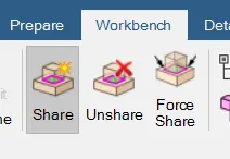
• Select share tool and enable share topology between two components

2.Meshing:

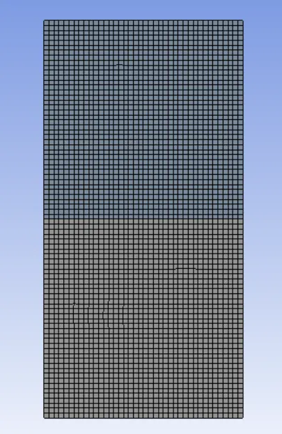
• Create base mesh

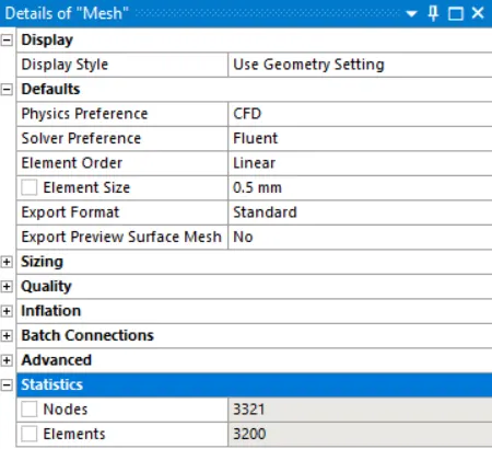
• Set mesh size to 0.5mm

3.Setup:

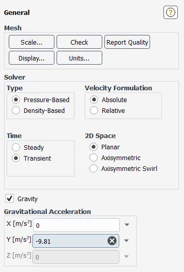
• Set solver as transient, Pressure-based and enable gravity

• Enable multiphase, under multiphase model select volume of fluid and implicit formulation

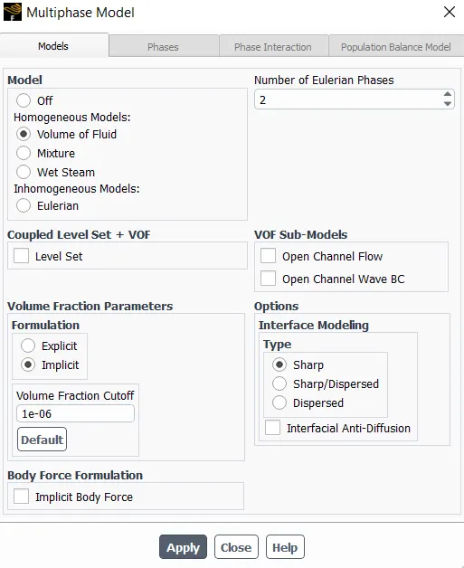
• Set number of eulerian phase to 2
• Add water as a material under create/change material tool
• Under multiphase model set air as primary phase and water as secondary phase
• Initialize the setup and select patch and set volume of water as 1 in water surface and 0 in air surface
• Create contour of volume of water, and create solution animation
• set the time step size and number of iterations and run the setup

Time-step size:0.025

4.Solution animation:

Refined case 1:

• Mesh size = 0.25
• Mesh detail:

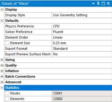
• Mesh:

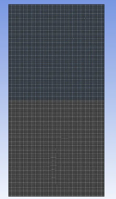
• Number of elements = 12800
• Solution:

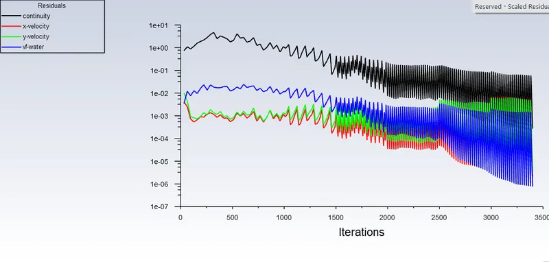
• Time step size: 0.01
• Solution animation:

Refined case 2:

• Mesh size = 0.2
• Mesh detail:

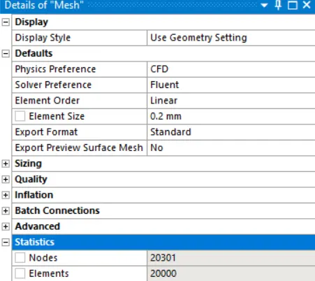
• Mesh:

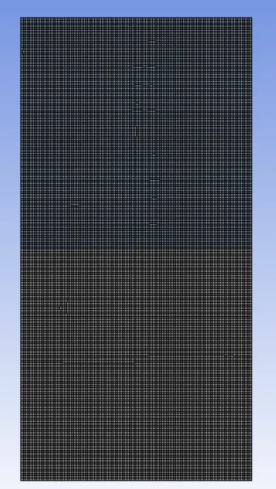
• Number of elements = 20000
• Mesh quality:

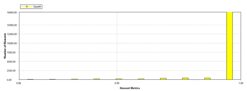
• Solution:
• Residuals:

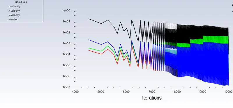
• Time step size: 0.005
• Solution animation:

Rayleigh-Taylor CFD simulation of water-user defined material for refined case:

User material properties:

• density = 400 kg/m3,
• viscosity = 0.001 kg/m-s

Create user defined material in create/edit material tool in Ansys fluent:

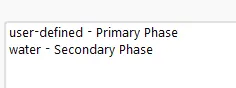
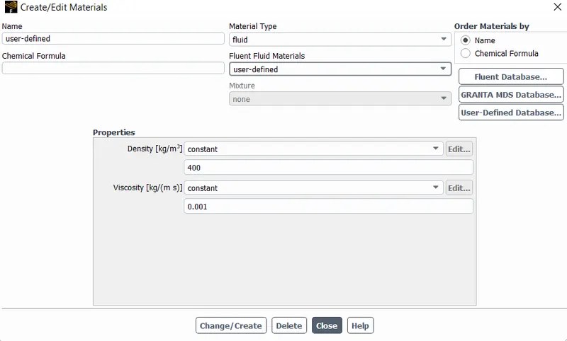Set primary phase as user defined material and secondary phase as water in multiphase setup

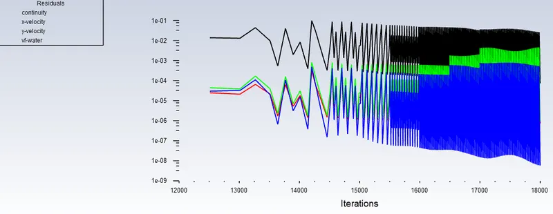
Residuals:

Solution animation:

Atwood number:

The difference in the fluid densities divided by their sum is defined as the Atwood number, A.

It is dimensionaless density ratio. It is giveb by:

`A = (rho1-rho2)/(rho1+rho2)`

where:

`rho1`= Density of heavier fluid

`rho2`= Density of lighter fluid

Atwood number for water-air and water-user defined material:

Water - air:

Given:

• `rho_(water) = 998.2 (kg)/(m^3)`
• `rho_(air) = 1.225(kg)/(m^3)`

`A = (rho_(water)-rho_(air))/(rho_(water)+rho_(air))`

`A = (998.2-1.225)/(998.2+1.225)`

`A = 0.9975`

Water - user material:

Given:

• `rho_(water) = 998.2 (kg)/(m^3)`
• `rho_(user) = 400(kg)/(m^3)`

`A = (rho_(water)-rho_(user))/(rho_(water)+rho_(user))`

`A = (998.2-400)/(998.2+400)`

`A = 0.4278`

Effect of Atwood number on behaviour of instability:

• For A close to 0, RT instability flows take the form of symmetric "fingers" of fluid.
• For A close to 1, the much lighter fluid "below" the heavier fluid takes the form of larger bubble-like plumes.

Water - air:

• Since the Atwood number is close to 1, we get bubble like plumes which we can see in solution animation.

Water - user material:

• Since the Atwood number is in between 0 and 1 we get the mixture of bubble like plumes and symmetric finger of fluid, As 0.4 is much closer to 0 than 1 , we can see from simulation we get more finger structures of fluid compared to water-air interface.

Conclusion:

• As we refine the mesh, the time step size needs to reduced to keep the solution stable.
• If the time step size are bigger than actual time RTI occurs, than instability grows in the solution, and the solution diverges giving floating point error.
• The finer the mesh, accurate are the results of simulation but simulation time increaes exponentially.