Week 5 - Rayleigh Taylor Instability

Objective :

In this challenge,

• We will discuss some practical CFD models that have been based on the mathematical analysis of Rayleigh Taylor waves and explain how these mathematical models have been adapted for CFD calculations.
• Perform the Rayleigh Taylor instability simulation for air and water with 2 different mesh sizes with mesh size 0.5 mm and 0.1mm and compare the results by showing the animations.We will observe the differences in the animation and explain the effect of mesh size on simulation and also, explain why a steady-state approach might not be suitable for these types of simulation.
• Then we run one more simulation with water and user-defined material(density = 400 kg/m³, viscosity = 0.001 kg/m-s) for refined mesh.
• Finally we define the Atwood Number and Find out the Atwood number for both the cases and explain how the variation in Atwood number in the above two cases affects the behavior of the instability.

Introduction :

Rayleigh–Taylor instability :

• The Rayleigh–Taylor instability, or RT instability (after Lord Rayleigh and G. I. Taylor), is an instability of an interface between two fluids of different densities which occurs when the lighter fluid is pushing the heavier fluid. Examples include the behavior of water suspended above oil in the gravity of Earth,mushroom clouds like those from volcanic eruptions and atmospheric nuclear explosions.
• The problem was governed by the Navier-Stokes and Cahn-Hilliard equations in a primitive variable formulation. The Cahn- Hilliard equations were used to capture the interface between two fluids
  systems.
• Water suspended on top oil is an everyday example of Rayleigh–Taylor instability, and it may be modeled by two completely plane-parallel layers of immiscible fluid, the more dense on top of the less dense one and both subject to the Earth's gravity. The equilibrium here is unstable to any perturbations or disturbances of the interface: if a parcel of heavier fluid is displaced downward with an equal volume of lighter fluid displaced upwards, the potential energy of the configuration is lower than the initial state. Thus the disturbance will grow and lead to a further release of potential energy ,as the more dense material moves down under the (effective) gravitational field, and the less dense material is further displaced upwards. This was the set-up as studied by Lord Rayleigh. The important insight by G. I. Taylor was his realisation that this situation is equivalent to the situation when the fluids are accelerated with the less dense fluid accelerating into the more dense fluid. This occurs deep underwater on the surface of an expanding bubble and in a nuclear explosion.
• As the RT instability develops, the initial perturbations progress from a linear growth phase into a non-linear growth phase, eventually developing "plumes" flowing upwards (in the gravitational buoyancy sense) and "spikes" falling downwards. In the linear phase, the fluid movement can be closely approximated by linear equations, and the amplitude of perturbations is growing exponentially with time. In the non-linear phase, perturbation amplitude is too large for a linear approximation, and mom-linear equations are required to describe fluid motions. In general, the density disparity between the fluids determines the structure of the subsequent non-linear RT instability flows (assuming other variables such as surface tension and viscosity are negligible here).
• The governing equations for The RTI problem are the Navier–Stokes equations, the continuity and the Cahn-Hilliard equations . in which which non-dimensional form of below eqations are used.

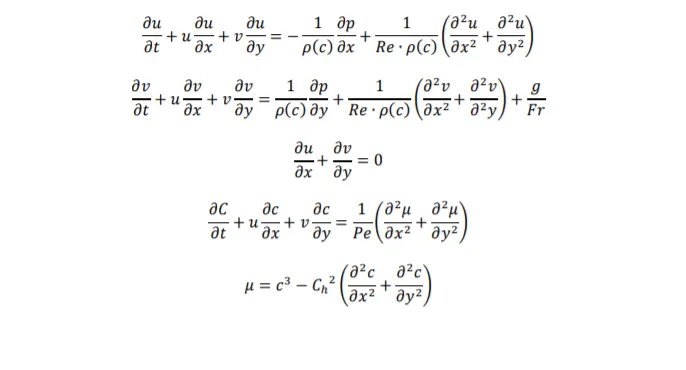
The evolution of the RTI follows four main stages. In the first stage, the perturbation amplitudes are small when compared to their wavelengths, the equations of motion can be linearized, resulting in exponential instability growth. In the early portion of this stage, a sinusoidal initial perturbation retains its sinusoidal shape. However, after the end of this first stage, when non-linear effects begin to appear, one observes the beginnings of the formation of the ubiquitous mushroom-shaped spikes (fluid structures of heavy fluid growing into light fluid) and bubbles (fluid structures of light fluid growing into heavy fluid). The growth of the mushroom structures continues in the second stage and can be modeled using buoyancy drag models, resulting in a growth rate that is approximately constant in time. At this point, nonlinear terms in the equations of motion can no longer be ignored. The spikes and bubbles then begin to interact with one another in the third stage. Bubble merging takes place, where the nonlinear interaction of mode coupling acts to combine smaller spikes and bubbles to produce larger ones. Also, bubble competition takes places, where spikes and bubbles of smaller wavelength that have become saturated are enveloped by larger ones that have not yet saturated. This eventually develops into a region of turbulent mixing, which is the fourth and final stage in the evolution. It is generally assumed that the mixing region that finally develops is self-similar and turbulent, provided that the Reynolds number is sufficiently large.Here ρ2 represents the heavy fluid and ρ1 represents the light fluid. Gravity is acting downward and the system is RT unstable.

Some practical CFD models that have been based on the mathematical analysis of Rayleigh Taylor waves :

Saffman–Taylor instability :

• The Saffman–Taylor instability, also known as viscous fingering, is the formation of patterns in a morphologically unstable interface between two fluids in a porous medium, described mathematically by Philip Saffman and G. I. Taylor in a paper of 1958.
• This situation is most often encountered during drainage processes through media such as soils. It occurs when a less viscous fluid is injected, displacing a more viscous fluid; in the inverse situation, with the more viscous displacing the other, the interface is stable and no instability is seen. Essentially the same effect occurs driven by gravity (without injection) if the interface is horizontal and separates two fluids of different densities, the heavier one being above the other: this is known as the Rayleigh-Taylor instability. In the rectangular configuration the system evolves until a single finger (the Saffman–Taylor finger) forms, whilst in the radial configuration the pattern grows forming fingers by successive tip-splitting.
• Most experimental research on viscous fingering has been performed on Hele-Shaw cells, which consist of two closely spaced, parallel sheets of glass containing a viscous fluid. The two most common set-ups are the channel configuration, in which the less viscous fluid is injected at one end of the channel, and the radial configuration, in which the less viscous fluid is injected at the centre of the cell. Instabilities analogous to viscous fingering can also be self-generated in biological systems.

Richtmyer–Meshkov instability (RMI) :

• The Richtmyer–Meshkov instability (RMI) occurs when two fluids of different density are impulsively accelerated. Normally this is by the passage of a shock wave. The development of the instability begins with small amplitude perturbations which initially grow linearly with time. This is followed by a nonlinear regime with bubbles appearing in the case of a light fluid penetrating a heavy fluid, and with spikes appearing in the case of a heavy fluid penetrating a light fluid. A chaotic regime eventually is reached and the two fluids mix. This instability can be considered the impulsive-acceleration limit of the Rayleigh–Taylor instability.

Plateau–Rayleigh instability :

• The Plateau–Rayleigh instability is named for Joseph Plateau and Lord Rayleigh. In 1873, Plateau found experimentally that a vertically falling stream of water will break up into drops if its wavelength is greater than about 3.13 to 3.18 times its diameter, which he noted is close to pi. Later, Rayleigh showed theoretically that a vertically falling column of non-viscous liquid with a circular cross-section should break up into drops if its wavelength exceeded its circumference, which is indeed π times its diameter.
• The Plateau–Rayleigh instability, often just called the Rayleigh instability, explains why and how a falling stream of fluid breaks up into smaller packets with the same volume but less surface area. It is related to the Rayleigh–Taylor instability and is part of a greater branch of fluid dynamics concerned with fluid thread breakup. This fluid instability is exploited in the design of a particular type of ink jet technology whereby a jet of liquid is perturbed into a steady stream of droplets.
• The driving force of the Plateau–Rayleigh instability is that liquids, by virtue of their surface tensions, tend to minimize their surface area. A considerable amount of work has been done recently on the final pinching profile by attacking it with self-similar solutions.

Kelvin–Helmholtz instability :

• The Kelvin–Helmholtz instability typically occurs when there is velocity shear in a single continuous fluid, or additionally where there is a velocity difference across the interface between two fluids. A common example is seen when wind blows across a water surface; the instability constant manifests as waves. Kelvin-Helmholtz instabilities are also visible in the atmospheres of planets and moons, such as in cloud formations on Earth or the Red Spot on Jupiter, and the atmospheres (coronas) of the Sun and other stars.

• When you see these models the instability of particular model will follow some trend of linear or non linear variation .So we can capture or denote these variation in some form of governing equations. then they can be adopted for CFD by solving the governing equations and other related flow equation that the instability denote.

Solution procedure :

• We wil simulate both fluid flow and also the heat transfer to the solid i.e., CHT Analysis on an Exhaust port with the steady state .Then for solving we follow the below procedure :

1)Geometry setup

2)Meshing

3) Problem setup

4)Solving

5)Post processing

Simulating the flow with the transient solver

Case-1 : Rayleigh–Taylor instability between air and water with coarse mesh of size 0.5 mm :

1) Geometry setup :

• In fluent module we have to open spaceClaim .
• At first, geometry is created as square boxes we are going to create square of dimensions 20 mm x 20 mm by using rectangle in spaceClaim and then convert it to surface by using Pull tool.After creating surface move it to a new component and name it as air .
• Then right click on the main design and create a new component and name it as water.Then again create a new square sketch of dimensions 20 mm x 20 mm by using rectangle over the previous created on on the same axis and next thing is as we need conformal mesh we need to use share in workbench and select both componens and click ok.Then you see share topology is also automatically set to share and you will see right icon modified and blue line is created at interface between them.
• The geometry was created in spaceclaim and it involves no other importing of CAD models. The surface model was further processed for meshing .This preprocessing phase of the workflow is extremely important because it determines the simulation potential and limits the CFD results.
• This completes the creation of geometry.Then we close the spaceClaim ,the progress will be saved automatically.

2) Meshing :

• For meshing we open Meshing,where we mesh our model so that we can use it to solve our model.
• In general it is always good to name the surfaces before meshing. So let us do that.
• We first select the entity by using the entity selection by using faces so that we can provide name for our entity selection.

steps : select the face you want to name by using face selection -> then press N -> name the selection.

• In the similar way we name the water side and air side.
• Then next thing to do is to mesh.We click the mesh option in the side then give element size as 0.5 mm and mesh.So this is our first case .

• Now we have to check the quality of the mesh.

steps : mesh ->quality-> mesh metric-> Element quality

• Here our minimum quality is around 15 %,so we can move further for our solution setup.

3) Problem Setup :

• To set up our problem we open Fluent and setup inital conditions , boundary conditions material etc.,
• We first start with checking the mesh quality using perform mesh check under domain.If no error is seen in console window then we can proceed further.
• Then we move move to setting up physics where we select the solver,viscous model etc.
• We use a transient state pressure based solver to solve our model.

Physics :

General :

Solver type : pressure based

time : transient state

velocity formulation : absolute

• We need to enable gravity by giving value for Y as -9.8 m/s^2 as gravity is acting in negative Y-direction.

models :

viscous model : Laminar (since the velocity is very small)

Material : Fluid -1 : Air

Fluid -2: Water

In models enable multiphase flow and in that select,

for model : select VOF method

Number of Eulerian phases : 2

Formulation : Implicit

• And in phases option as we selected two phases give names and selcect phase ,
• For primary phase :change name as air and change phase material to air
• For secondary phase :change name as water and change phase material to water.
• Then for doing patching we have to initialize first and then we do Hybrid initialization .
• In patch for phase select water and for variable you can see volume fraction now .
• Now, patch the value fraction value of 0 to air side and 1 to water side.(i.e., at t=0 the top box will be total water and bottom box will be total air.)
• Now we are almost ready to run the simulation but as to verify the patching,we create contour for volume fraction of water .
• Now we want to see the volume fraction of water contour.
• For contour -> go to solutions tab -> graphics -> contour -> in contour of : select phases and under that select volume fraction and for phase select water -> select both the boxes or surfaces and press save /display.
• Then you can see the initial values for volume fraction of water on whole domain,where you can see in the bottom it is set to 0 and for the top region it is set to 1.So we can conclude that our initialization is correct.
• Then we want to create animation so that we can see how the solution or volume fraction of water is is varying when problem is being solved.
• For that,

steps : Activities -> solution animation -> select volume fraction contour,which we have created -> preview -> set the required view and use active -> and name it as volume fraction of water animation.

• Then in solution method for Pressure velocity coupling SIMPLE scheme is used. For the momentum second order upwind scheme is used and for pressure, PRESTO is selected. For the transient formulation first order implicit scheme is choosen for better results and for stability and convergence of the residuals.
• Then we are ready to solve .

4) Solving :

• Give iterations and time step such that solution is converged.
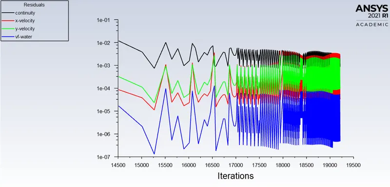
• Run the simulation until the steady state is reached.Lets run for 1300 times steps with time step size = 0.005 and the total run time =6.5 s .
• we can find the solution is converged.
• If you see error of diverging solution ,then try to under relax or try to use lower order discretization schemes so that we can ge converged solution.
• Then let us post process the results.

5)Post processing :

Residuals plot :

• You can observe from the below plot the residuals has converged.

Animation :

• Animation of Rayleigh–Taylor instability between air and water with coarse mesh.

Volume fraction of water contour :

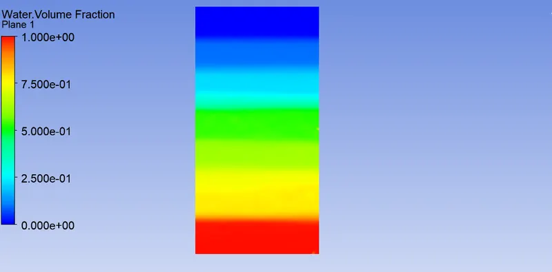
• You can observe from the below contour the volume fraction of water.

Case- 2 :Rayleigh–Taylor instability between air and water with fine mesh of size 0.1 mm :

• Everything is same from the point of geometry and when it comes to mesh the only change is the mesh size,here it is quite refined with mesh size of 0.1 mm.
• Comming to set up even it is also same.
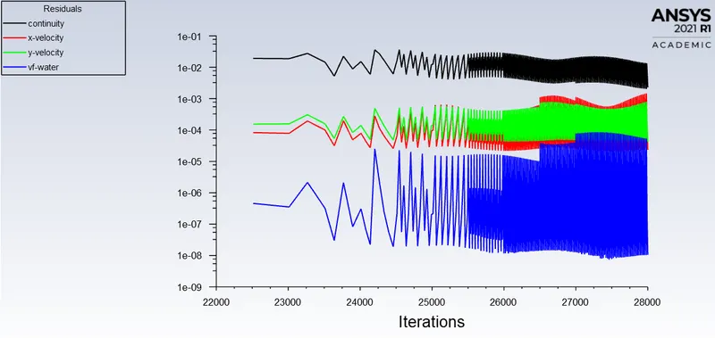
• Here we run for 1400 times steps with time step size = 0.005 and the total run time = 7s.
• So let us directly run the simulation then postprocess the results and compare in between the results of two different grid sizes .

Residuals plot :

• You can observe from the below plot the residuals has converged .

Animation :

• Animation of Rayleigh–Taylor instability between air and water with finer mesh.

Volume fraction of water contour :

• You can observe from the below contour the volume fraction of water.

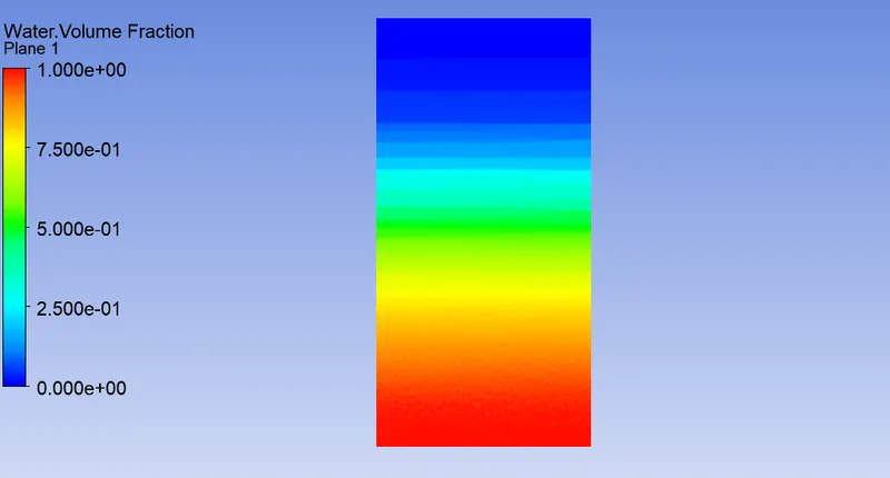
• You can observe the volume fraction of the same problem but the mesh is even more refined(0.07 mm).Here the numerical diffusion(due to low order scheme used for convergence)is even more less ,we get some more accurate result than above.So small the grid size more the computational effort and more the accurate solution the result is.

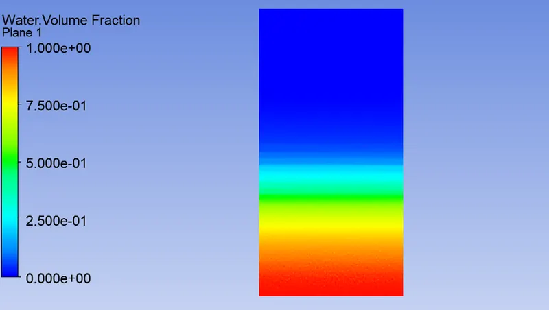
• For Case -1 the transient case was run for 1300 time steps with a time step size of 0.005 We can observe from the water volume fraction how the air has moved upwards while the water settles down. For Case 2 this case was ran for1400 time steps with a time step size of 0.005. As the mesh size is refined we get more defined results which we can see from the above plots and animations and also it took a long time for the simulation to reach appropriate results.
• At first the fluids behave linearly and we can observe small linearity sinking going on between them, slowly the chunky bubbles from the higher density fluid on top settles down. This can be identified from the highest mesh case resulting in finest behaviour of the instability for this condition. Atfirst very small time, the small enough, initial perturbation in flow can be described by a smooth function. We observe the disturbance in flow from smooth to turbulent growth has been observed as we go through time. We also observed the transition of a single globule into lots of deformed globules with with lots of turbulence along with some breakup and penetration of heavier fluid into the lighter one. These breakups which seems at initial stage vanishes as time proceed as in showing the phenomena of Rayleigh-Taylor instability.
• At middle time, it is clear that the falling fluid is rolled up. In our result, finally the heavier fluid has settled down completely at t = 7 s or we can say it is in the verge of complete settling. Above animations shows 2D-Rayleigh Taylor Instability simulation having the contours of two phase mixture model. It shows the penetration of heavier fluid into lighter fluid with the progress of flow time. For time,t ≥ 1.5, the simulation enters the non-linear regime with the increase in amplitude of perturbation. At later time we observe the formation of low density bubbles and its rise into the high density phase whereas the high density globules sinks at the edges of the domain of the simulation into the light fluid.
• With the time evolution, the interface gets smeared due to numerical diffusion within the interfaces. The shape of the globules deforming as flow time progresses actually varies with the meshing.
• The volume fraction in simulations on different meshes at a particular flow time shows the interface thickness is smaller on finer mesh.So finer the mesh we can see the better volume fraction contour but with an expense of computational effort.

In the current problem or simulation steady-state approach might not be suitable .For these types of simulation always we have to use transient simualtion because the problem is in transient in nature and we can see how the instability is varying and how the intreface is changing clearly when we use transient simulation.When we use steady state we only get the final result which is correct and we cannot see whats happening with respect to time.So our main here is to simulate how the instability is happening with respect to time ,so we have to use transient simulation.Smaller time steps are required to observe the instabilities and can be only possible through transient simulation. Since it is a time marching solution, we expect more accuracy from transient simulation for which Transient simuation is the ideal setup to run the calculation for Rayleigh Taylor Instability.

Case- 3 :Rayleigh–Taylor instability between user defined material and water with fine mesh of size 0.1 mm :

• Everything is same from the point of geometry and even when it comes to mesh, the mesh size is also same as refine case above i.e., 0.1 mm.
• Comming to setup the change comes here ,we change the lighter material i.e.,from air to user defined material with density = 400 kg/m³, viscosity = 0.001 kg/m-s .
• Then again every thing is same ,we patch the lighter fluid down and denser fluid upper side of the box or domain.
• Then we run for 1800 times steps with time step size = 0.005 and the total run time = 9.00s.
• So let us directly run the simulation then postprocess the results and compare the results with above case -2 with respect to Atwood number .

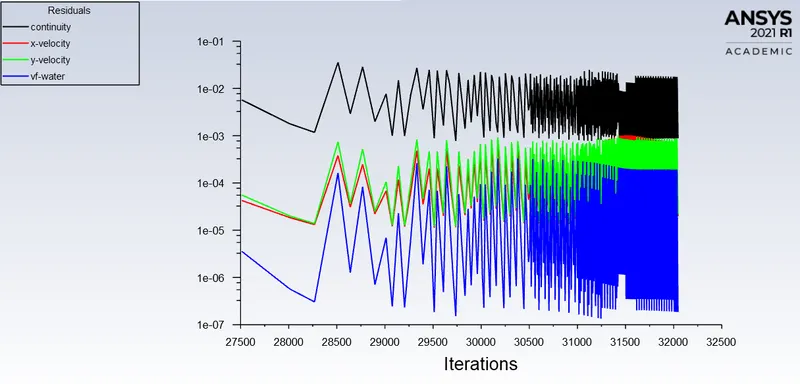
Residuals plot :

• You can observe from the below plot the residuals has converged .

Animation :

• Animation of Rayleigh–Taylor instability between user defined material and water with finer mesh.

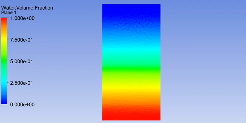
Volume fraction of water contour :

• You can observe from the below contour the volume fraction of water.

Atwood number :

In fluid dynamics, the Atwood number (A) is a dimensionless-number.The Atwood number is defined as a dimensionless density ratio it is given as:

Formula:

Significance :

• The Atwood Number is a dimensionless number in Fluid Dynamics. It is used in the study of instabilities of the dynamics of the fluid flow.It gives the relation between density of higher fluid and the density of lighter fluid
• The Atwood number is used in the study of Rayleigh Taylor instability.
• The Rayleigh–Taylor instability, is an instability of an interface between two fluids of different densities, which occurs when the lighter fluid is pushing the heavier fluid.For example, when the water is suspended above oil in the gravity.
• For Atwood number closer to 1,means the lighter fluid below the heavier fluid takes the form of larger bubble-like plumes.
• Let us find Atwood number for both the above cases and explain how the variation in Atwood number in the above two cases affects the behavior of the instability.

Atwood number for both the above cases :

• For case-1 i.e., Atwood number for air and water =(998.2-1.225)/(998.2+1.225) = 0.9975
• For case-2 i.e., Atwood number for user defined material or fluid and water =(998.2-400)/(998.2+400) = 0.4278

Effect of variation of Atwood number in the above two cases on the behavior of the instability :

• We observe that the evolution of the interface grows faster with the increase in Atwood Number for which in this study the Atwood Number is kept as high as possible in Case 2. It was seen that with larger Atwood Number, larger amplitude of perturbations are observed. It is due to the larger density ratio of the two fluids, the stronger is the force to develop the interface instability.. For Atwood no. close to 0, RT instability flows takes the form of symmetric "fingers" of fluid.In lower Atwood numbers i.e.,in case -3 ,spikes and globules were still present at the end of the simulation.
• With the decrease in Atwood Number from Case 2 to 3 from 0.99 to 0.42 respectively and when compared, we can clearly observe from that bubbles and spikes formation are still present at the same flow time or even after completion of simulation or at the verge of settling.The formation is because of the increase in density of secondary phase with a density of for Case-3. For the case of smaller Atwood Number, the density difference between the two sides of the interface is small and the density distribution of the upper and lower layers is nearly symmetrical.
• The initial density stratification plays a dominant role and the expansion compression effect has a little influence. With the increased Atwood Number close to 1 the stabilization effect of initial density stratification decreases and the instability caused by the expansion-compression effect becomes more significant. It can be seen in the animation that the larger Atwood numbers, the larger amplitude ofperturbation. It takes place due to the larger density ratio of two fluids is, the stronger force to develop the interface instability. The flow structure of bubbles and globules are quite different both for the variation in meshing and also with the variation in Atwood Number.
• The increase of Atwood number, the time of spikes or globules of the denser phase fluid arriving at the bottom of the computational domain is accelerated, then the duration of RTI in the steady growth stage is shorter. We can observe that the compressibility on the bubble velocity is strong at larger Atwood Number. The bubble height is approximately a quadratic function of time at potential flow growth stage. The average bubble acceleration is nearly proportional to the square of the Mach Number of Atwood Number close to 1. For Atwood No. close to 1, the much lighter fluid below the heavier fluid takes the form of larger bubble like plumes.Since in our simulation for case-2 has Atwood Number close to 1 ,lighter fluid takes bubble form and thus helping in validating that our simulation is correct.

Conclusions :
In the present challenge, classical method of FVM was adopted to study the evolution of the interface during RTI. The governing equations were Navier-Stokes equations and Cahn-Hilliard equations.Steady state solution determines the fully developed solution. This numerical simulation was validated with the observations obtained by previous researchers and this was done by the variation in Atwood Number where we obtained the same observation. In lower Atwood numbers, spikes and globules were still present at the end of the simulation which was not there in Atwood Number of 0.99 in Case -2 . From the grid dependency we also observed that the interface thickness reduces with the refined mesh.For Transient simulation,compared to steady state, has higher demand in terms of computational time. Transient solver better captures the flow and can be used to run at smaller time steps with a time step size of 0.005. Smaller time steps are required to observe the instabilities and can be only possible through transient simulation. Since it is a time marching solution, we expect more accuracy from transient simulation for which Transient simuation is the ideal setup to run the calculation for Rayleigh Taylor Instability.