Week 9 - FVM Literature Review

Finite Volume Method (FVM):

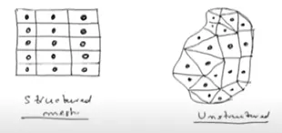
• The finite volume method is based on the approximate solution of the integral form of the conservation equations. The problem domain is divided into set of non-overlapping control volumes called finite volumes. The conservation equations are applied to each finite volume. Integrals occurring in the conservation equations are evaluated using functional values at computational nodes.
• FVM can accommodate any type of grid and hence it is naturally suitable for complex geometries. This explains its popularity for commercial CFD packages, which must cater to problems in arbitrarily complex geometries.

Solution process:

• Discretize the solution domain by a grid and define the computational nodes at which variables are to be evaluated.
• Then apply the integral form of conservation law to each finite volume.
• Approximate the surface and volume integrals using the appropriate quadrature formulae in terms of the function values at computational nodes.
• Collect the algebraic equations for all the finite volumes to obtain a system of algebraic equations in terms of unknown values of the variable at computational nodes.
• Solve the resulting system of algebraic equations depending on the nature of the system, we can solve by using a linear solver or non-linear solver to obtain the values of the variable at each computational node.

Classification: On the choice of computational nodes FV grids are classified t two common approaches.

• Cell - centered approach: CVs are defined by a suitable grid and computational nodes are assigned at the CV Centre. It can be used with structured or unstructured grids.

• Face - centered approach: Nodal locations are defined first, and CVs are then constructed around them so that cv faces lie midway between the nodes. It can be only used with structured grids.

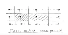
Hence cell-centered approach is more commonly used.

Compass Notation:

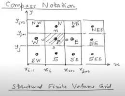
• For structured cartesian grids, compass notation is employed for computational nodes. Nodes denoted by upper case letters P, E, W, N, S, T, B.
• Plane faces denoted by lower case letters corresponding to their direction (e, w, s, n, t and b) with respect to the central node P.

Difference between FDM and FVM:

• Finite difference method uses differential form of equations whereas in FVM we use integral form of equations.
• You cannot use FDM directly when the grids are not aligned in X, Y or Z direction. This is the major drawback.
• Whereas in FVM you can handle any type of geometry.
• FDM cannot handle discontinuous in domain where as FVM can do it.
• FVM preserves the conservative properties where as FDM don’t.

Interpolation methods:

The approximation of surface and volume integrals require value of variable at location other than computational nodes of the CV. Values at these locations are obtained using interpolation formulae.

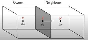
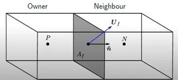
Each face connects an owner cell(P) and a neighbor cell(N). We don’t care about the number of faces here. Hence the analysis valid for all polyhedral cells. The boundary faces and internal faces require different treatment. Assume that we know the value of some quantity ϕ on the owner centroid (ϕP) and the neighbour cell centroid (ϕN). ϕ could be any field T,p,U etc.We want to know ϕf.

The different types of interpolation schemes are

1) Upwind differencing scheme (UDS) :

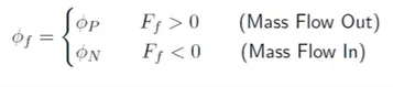
• The upwind differencing depends upon the direction of the mass flux.
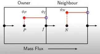
• UDS is equivalent to using a backward or forward finite different approximation depending upon the flow direction.

• The value of the ϕ on the cell face (ϕf) is given by

• ϕ is constant between the cell centroid and cell face it will not varies linearly.Hence upwind difference is only first order accurate.

Advantage :

• UDS is the only approximation that satisfies boundedness criterion unconditionally.
• It is the most stable scheme for convection dominated flows.
• We can use to generate an initial ,stable solution.

Disadvantages :

• UDS is not accurate.It is numerically diffusive.
• Peaks or rapid variations in the variables will be smeared out.
• As it is only first order accurate hence very fine grids are required to obtain accurate solution.

2) Linear Interpolation / Central Differencing scheme (CDS) :

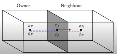
• Approximate the value of variable at CV face centre by linear interpolation of the values at two nearest computational nodes.
• The linear interpolation is equivalent to the use of central differnce formula of the first order derivative,and hence,this is also termed as central difference scheme(CDS).

Characteristics :

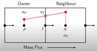
• As the variations between centroid is linear, CDS scheme is second order accurate.
• The scheme is unbounded,it may produce oscillatory solutions.It is simplest and most widely used interpolation.
• Leads to a very simple approximation for evaluations of gradients required for evaluation of diffusive fluxes.
• Approximation of gradients has second order accuracy on uniform grids.It's formally first order on non-uniform grids.

3)Quadratic Upwind Interpolation (QUICK) :

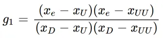
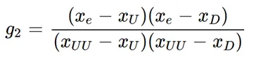
• Approximate the value of the variable at CV face centre by quadratic interpolation of the values at three nearest computational nodes (one downstream node D and two upstream nodes U,UU).
• It is third order accurate for both uniform and non uniform grids.

where,

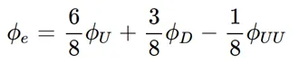
• On uniform grids, its simplified form is,

4)Linear Upwind Differencing:

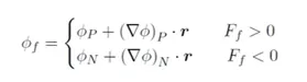
• Linear upwind differencing is a popular scheme.
• It is more accuratethan upwind differencing.
• We use the gradient (∇ϕ) to improve the accuracy of extrapolation.
• Linear upwind differencing is popular for the convection term.

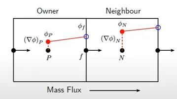
• The variation between the cell centroid and the face is linear, Hence the scheme is nominally second order accurate.

5) Hybrid Interpolation Scheme:

• It is a blend of CDS for accuracy and UDS scheme for stability based on local peclet number.

Gradient schemes:

• The gradient schemes are used to find the gradient. A gradient is a vector of 3 components.
• In a CFD code gradient is used for,
• In interpolation schemes like Linear upwind scheme.
• We need them for non-orthogonal correctors.
• In some source terms gradient is used in order to evaluate them etc.

flux limiters:

• In higher order schemes the flux limiter limit the solution near the shocks instead of allowing it to grow and blow the solution.
• Let’s see below figure to get more clarity on what flux limiter is,

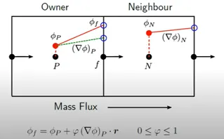
• Here the gradient is limited instead of allowing it to grow which is shown by a green dotted line so that it is bounded.