Week 12 - Validation studies of Symmetry BC vs Wedge BC in OpenFOAM vs Analytical H.P equation

Objective :

In this challenge ,we will simulate an axi-symmetric flow through a cylinderical pipe by applying both wedge and Symmetry Boundary Condition .We will do the simulation with different angles i.e., 10,25 and 45 degrees .Simulating flow through a pipe will be computationally costly ,so as the flow through a pipe is axi-symmetric in nature we will split the domain and simulate only for the sector of the domain considering a wedge portion .Here we are simulating the Hagen poiseuille's flow which is an incompressible laminar flow occuring through a through a constant cross-section smooth cylinderical pipe and we consider an inlet Reynold's number of as 2100.We will do transient state simulation and validate our results with the Hagen- Poiseuille's flow equations for the fully developed flow.Here we will write a code in Matlab to automate the generation of blockMeshDict file and use it in OpenFoam. The following are the results we will show in this project and validate the results that are obtained with both wedge and symmetry Boundary Condition with analytical solution i.e, by Hagen poiseuille's flow equations,

• We will validate Hydro-dynamic length from Hagen poiseuille's flow with the numerical result.
• Then validate the fully developed flow velocity profile with its analytical profile by Hagen poiseuille's flow equations.
• We then validate maximum velocity and pressured drop for fully developed flow.
• Post-process Shear stress and validate wall shear stress for fully developed flow.
• Highlight the differences in both boundary conditions in terms of their usage and application.

Theory :

The Hagen–Poiseuille equation, also known as the Hagen–Poiseuille law, Poiseuille law or Poiseuille equation, is a physics law that gives the pressure drop in an incompressible and Newtonian fluid inlaminar flow flowing through a long cylindrical pipe of constant cross section.

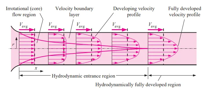
Consider a fluid entering a circular pipe at a uniform velocity. Because of the no-slip condition, the fluid particles in the layer in contact with the surface of the pipe come to a complete stop. This layer also causes the fluidparticles in the adjacent layers to slow down gradually as a result of friction.To make up for this velocity reduction, the velocity of the fluid at the mid-section of the pipe has to increase to keep the mass flow rate through thepipe constant. As a result, a velocity gradient develops along the pipe.The region of the flow in which the effects of the viscous shearing forces caused by fluid viscosity are felt is called the boundary layer.

The hypothetical boundary surface divides the flow in a pipe into two regions: the boundary layer region, in which the viscous effects and the velocity changes are significant, and the irrotational (core) flow region, in which the frictional effects are negligible and the velocity remains essentially constant in the radial direction. The thickness of this boundary layer increases in the flow direction until the boundary layer reaches the pipe center and thus fills the entire pipe, as shown in below figure. The region from the pipe inlet to the point at which the boundary layer merges at the centerline is called the hydrodynamic entrance region, and the length of this region is called the hydrodynamic entry length L_h.

Flow in the entrance region is called hydrodynamically developing flow, since this is the region where the velocity profile develops. The region beyond the entrance region in which the velocity profile is fully developed and remains unchanged is called the hydrodynamically fully developed region.

Operating conditions and Analytical solution :

Reynolds Number :The transition from laminar to turbulent flow depends on the geometry, surface roughness, flow velocity, surface temperature, and type of fluid, among other things.The flow regime depends mainly on the ratio of inertial forces to viscous forces in the fluid. This ratio is called the Reynolds number and is expressed for internal flow in a circular pipe as

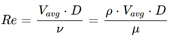
where Vavg = average flow velocity (m/s),rho =density, D = characteristic length of thegeometry (diameter in this case, in m), and nu = mu/rho = kinematic viscosity of the fluid (m2/s). Note that the Reynolds number is a dimensionless quantity. Also, kinematic viscosity has the unit m2/s, and can beviewed as viscous diffusivity or diffusivity for momentum.

Hydrodynamic entry length :

since the flow is laminar ,The hydrodynamic entry length is given as, L_h = 0.05*Re*D.

Velocity profile and Average velocity :

The velocity profile in fully developed laminar flow in a pipe is parabolic with a maximum at the centerline and minimum (zero) at the pipe wall.

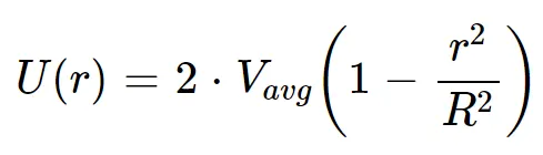
This is a convenient form for the velocity profile since V_avg can be determined easily from the flow rate information. The maximum velocity occurs at the centerline and is determined from
above equation by substituting r = 0,

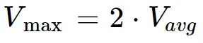
Average velocity,V_avg is defined as the average speed through a cross section. For fully developed laminar pipe flow, V_avg is half of maximum velocity.In fluid flow, it is convenient to work with an average velocity V_avg, which remains constant in incompressible flow when the cross-sectional area of the pipe is constant.Also from the definition of renold's number we can get the average velocity.

Pressure drop(ΔP) : The Pressure gradient shows the difference in the pressure between the two ends of the tube , determined by the fact that any fluid will always flow from high pressure to low pressure region and the flow rate is determined by the pressure gradient.Here as the Hagen poiseuille's equation is valid only for fully developed flow we will consider the pressure difference between the hydrodynamically fully developed region.

R= Radius of tube .The liquid flow varies directly with the radius.

Viscosity( μ) : The flow of the fluid varies inversely with the viscosity of the fluid and as the viscosity of the fluid increases, the flow decreases vice versa.
Length of the Tube (L): The liquid flow is inversely proportional to the length of the tube, therefore longer the tube, greater is the resistance to the flow.

Solution procedure :

• First we start by calculating the Analytical Solution for flow variables by Hagen–Poiseuille equations from the above mentioned equations .These are useful to validate our numerical solution and also we give initial conditions based on these values .
• Then comming to Numerical solution we start with writing a code in Matlab to automate the generation of blockMeshDict file for different angles and different boundary conditions to use it in OpenFoam.
• Then as the flow is laminar and incompreesible we use the solver IcoFoam which solves laminar incompressible navier stokes equations.Then we select a tutorial under IcoFoam i.e,cavity then we replace the existing BlockMeshDict file which was present , with the BlockMeshDict file which we created in matlab.
• Then we give the initial conditions for pressure and velocity by editing the p and U file in 0 folder.
• As the working fluid is water we change the kinematic viscosity which is already present with kinematic viscosity of water which is present in transport properties under constant folder.
• Then we change the time step and time in the controlDict file such that the simulation is stable and perfectly executed.
• Then we run the solver IcoFoam and and plot the results.
• The same procedure is repeated for different wedge angles and with wedge and symmetry boundary conditons.
• And finally we validate them with analytical solution i.e, by Hagen poiseuille's flow equations.

Analytical Solution for flow variables by Hagen–Poiseuille equation :

Hence to find the analytical solution we need to have the properties of working fluid i.e, here water ,and the pipe dimensions and flow conditions.Therefore lets consider ,

• Diameter of pipe, D =0.02m
• radius of pipe, r= D/2= 0.01m
• Reynolds's number , Re =2100
• Wedge angle, theta =we try with 10,25,45 degrees
• Density of water, rho = 997 kg/m^3
• Dynamic viscosity of water ,mu = 8.9*1e-4 Pa.s
• kinematic viscosity, nu = mu/rho= 8.9268e-07 m^2/s

Now from the Hagen–Poiseuille flow conditions we get,

• Hydrodynamic entry length,L_he = 0.05*Re*D

L_he =0.05*2100*0.02 =2.1m

• Length of pipe, L_p =L_he+1

L_p =2.1+1 =3.1m

• Average velocity, V_avg = Re*nu/D

V_avg = 2100*8.9268e-07/0.02 = 0.0937 m/sec

• Maximum velocity ,V_max =2*V_avg

V_max = 2*0.0937 = 0.1875 m/sec

• Pressure drop,ΔP = (8*V_avg*mu*L_p)/(r^2)

del_P(ΔP) = (8*0.0937*8.9*1e-4*1)/(0.01)^2 = 6.6737 Pa

(Here as the Hagen poiseuille's equation is valid only for fully developed flow we will consider the pressure difference between the hydrodynamically fully developed region. i.e,L_p =1m)

• Since here OpenFoam deals with kinematic pressure ,k_P =del_P/rho

k_P = 6.6737/997 = 0.0067 m^2/sec^2

Numerical Solution :

We start with writing a code in Matlab which automatically creates the vertices by the wedge angle that we specify.Here the geometry we create is wedge which is made of single block.This code then automate the generation of blockMeshDict file to use it in the OpenFoam.This code also gives the analytical solution and initial conditions for the simulation by taking above initial values and operating conditions by solving Hagen poiseuille's flow conditions.

Matlab code :

clear all
close all
clc

Re =2100 ;% reynolds's number
D =0.02 ; %diameter of pipe in metres
r= D/2; % radius of pipe
theta = 10; %Wedge angle 
L_he = 0.05*Re*D; %Hydrodynamic entry length
L_p =L_he+1; % length of pipe
rho = 997;   %density of water kg/m^3
mu = 8.9*1e-4;   %dynamic viscosity of water in Pa.s      
nu = mu/rho; %kinematic viscosity in m^2/s
L =1 ;   %Length of hydrodynamically fully developed region.
V_avg = Re*nu/D;  %Average flow velocity in m/sec
V_max =2*V_avg; %maximum velocity in m/sec
del_P = (8*V_avg*mu*L)/(r^2); %pressure drop
k_P =del_P/rho; %kinematic pressure drop m^2/sec^2
% vertices
V_0 =[0 0 0];
V_1 =[0 r*cosd(theta/2) r*sind(theta/2)];
V_2 =[0 r*cosd(theta/2) -r*sind(theta/2)];
V_3 =[L_p 0 0];
V_4 =[L_p r*cosd(theta/2) r*sind(theta/2)];
V_5 =[L_p r*cosd(theta/2) -r*sind(theta/2)];

% creating blockMeshDict file for openFoam

header{1}='/*--------------------------------*- C++ -*----------------------------------*\';
header{2}='  =========                 |                |';
header{3}='  \\      /  F ield         | OpenFOAM: The Open Source CFD Toolbox';
header{4}='   \\    /   O peration     | Website:  https://openfoam.org';
header{5}='    \\  /    A nd           | Version:  8';
header{6}='     \\/     M anipulation  |';
header{7}='\*---------------------------------------------------------------------------*/';

 f1 = fopen('week12_3(45deg).txt','wt');
 for i =1 :length(header)
fprintf(f1,'%s\n ',header{i});
 end
 
 fprintf(f1,'\n');
fprintf(f1,'%s\n','FoamFile');
fprintf(f1,'%s\n','{');
fprintf(f1,'%16s% 10s\n','version' ,' 2.0;');
fprintf(f1,'%16s %12s\n',' format' ,' ascii;');
fprintf(f1,'%16s %17s\n','class ','dictionary;');
fprintf(f1,'%16s %20s\n','object', 'blockMeshDict;');
fprintf(f1,'%s\n\n',' }');
fprintf(f1,'%s\n','// * * * * * * * * * * * * * * * * * * * * * * * * * * * * * * * * * * * * * //');
fprintf(f1,'%s\n','convertToMeters 1;');
fprintf(f1,'\n');
% vertices
fprintf(f1,'%s\n','vertices');
fprintf(f1,'%2s\n','(');
fprintf(f1,'\t(%d %d %d)\n',V_0);
fprintf(f1,'\t(%d %d %d)\n',V_1);
fprintf(f1,'\t(%d %d %d)\n',V_2);
fprintf(f1,'\t(%d %d %d)\n',V_3);
fprintf(f1,'\t(%d %d %d)\n',V_4);
fprintf(f1,'\t(%d %d %d)\n',V_5);
fprintf(f1,'%2s\n\n',');');

% defining the block
z=[300 50 1]; %no of cells in X,Y and Z direction
d=[0.2 1 1 ];  %simple grading
fprintf(f1,'blocks \n (\n');
fprintf(f1,'\t%s (%d %d %d) %s (%d %d %d)','hex (0 3 5 2 0 3 4 1)',z,'simpleGrading',d);
fprintf(f1,'\n\n%2s',');');

fprintf(f1,'\n%s\n','edges');
fprintf(f1,'%s\n','(');

fprintf(f1,'%s\n','arc 1 2 (0 0.01 0)');
 fprintf(f1,'%s\n','arc 4 5 (3.100000e+00 0.01 0)');
fprintf(f1,'%s\n',');');
% defining boundaries
fprintf(f1,'%s\n','boundary');
fprintf(f1,'%s\n','(');
%inlet
fprintf(f1,'\t%5s\n','inlet','{');
fprintf(f1,'\n%17s %s\n', 'type', 'patch;');
fprintf(f1,'%18s \n\t %s\n','faces','(');
fprintf(f1,'%24s \n%11s \n\n%15s\n\n','(0 1 2 0)',');','}');
% outlet
fprintf(f1,'\t%5s\n','outlet','{');
fprintf(f1,'\n%17s %s\n', 'type', 'patch;');
fprintf(f1,'%18s \n\t %s\n','faces','(');
fprintf(f1,'%24s \n%11s \n\n%15s\n\n','(3 5 4 3)',');','}');
% top wall
fprintf(f1,'\t%5s\n','topWall','{');
fprintf(f1,'\n%17s %s\n', 'type', 'wall;');
fprintf(f1,'%18s \n\t %s\n','faces','(');
fprintf(f1,'%24s \n%11s \n\n%15s\n\n','(1 4 5 2)',');','}');
%bottom axis
fprintf(f1,'\t%5s\n','bottomAxis','{');
fprintf(f1,'\n%17s %s\n', 'type', 'empty;');
fprintf(f1,'%18s \n\t %s\n','faces','(');
fprintf(f1,'%24s \n%11s \n\n%15s\n\n','(0 3 3 0)',');','}');
% wedge front
fprintf(f1,'\t%5s\n','wedgeFront','{');
fprintf(f1,'\n%17s %s\n', 'type', 'symmetry;');
fprintf(f1,'%18s \n\t %s\n','faces','(');
fprintf(f1,'%24s \n%11s \n\n%15s\n\n','(3 4 1 0)',');','}');
% wedge back
fprintf(f1,'\t%5s\n','wedgeBack','{');
fprintf(f1,'\n%17s %s\n', 'type', 'symmetry;');
fprintf(f1,'%18s \n\t %s\n','faces','(');
fprintf(f1,'%24s \n%11s \n\n%15s\n\n','(2 5 3 0)',');','}');
fprintf(f1,');\n\n');
% mergepatchpairs
fprintf(f1,'mergePatchPairs\n');
fprintf(f1,'(\n');
fprintf(f1,');\n\n\n');

fprintf(f1,'// ************************************************************************* //');

fclose(f1);

The code below is the blockMeshDict text file which was generated by Matlab.Then we replace the existing BlockMeshDict file which was present , with the BlockMeshDict file which we created in matlab in the OpenFoam.In the above code the the only thing we change is wedge angle for simulation which we do for different angles ,and based upon that only the vertices will be changed remaining everything is constant for each of the simulation we do now, but one thing we also change is the boundary condition for wedgeFront and wedgeBack ,depending upon the problem, we change in between wedge and symmetry.

BlockMeshDict file :

/*--------------------------------*- C++ -*----------------------------------*\
   =========                 |                |
   \\      /  F ield         | OpenFOAM: The Open Source CFD Toolbox
    \\    /   O peration     | Website:  https://openfoam.org
     \\  /    A nd           | Version:  8
      \\/     M anipulation  |
 \*---------------------------------------------------------------------------*/
 
FoamFile
{
         version      2.0;
          format       ascii;
          class        dictionary;
          object       blockMeshDict;
 }

// * * * * * * * * * * * * * * * * * * * * * * * * * * * * * * * * * * * * * //
convertToMeters 1;

vertices
 (
	(0 0 0)
	(0 9.961947e-03 8.715574e-04)
	(0 9.961947e-03 -8.715574e-04)
	(3.100000e+00 0 0)
	(3.100000e+00 9.961947e-03 8.715574e-04)
	(3.100000e+00 9.961947e-03 -8.715574e-04)
);

blocks 
 (
	hex (0 3 5 2 0 3 4 1) (300 50 1) simpleGrading (2.000000e-01 1 1)

);
edges
(
arc 1 2 (0 0.01 0)
arc 4 5 (3.100000e+00 0.01 0)
);
boundary
(
	inlet
	    {

             type patch;
             faces 
	 (
               (0 1 2 0) 
         ); 

              }

	outlet
	    {

             type patch;
             faces 
	 (
               (3 5 4 3) 
         ); 

              }

	topWall
	    {

             type wall;
             faces 
	 (
               (1 4 5 2) 
         ); 

              }

	bottomAxis
	    {

             type empty;
             faces 
	 (
               (0 3 3 0) 
         ); 

              }

	wedgeFront
	    {

             type symmetry;
             faces 
	 (
               (3 4 1 0) 
         ); 

              }

	wedgeBack
	    {

             type symmetry;
             faces 
	 (
               (2 5 3 0) 
         ); 

              }

);

mergePatchPairs
(
);


// ************************************************************************* //

The below are the vertices for 25 degrees and 45 degrees respectively,

Vertices for 25 degrees :

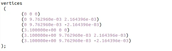
Vertices for 45 degrees :

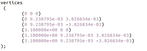
Then we will give the initial and boundary conditions for pressure and velocity by editing the p and U file in 0 folder.In the below presssure and velocity everything is constant for each of the simulation we do now, but one thing we change is the boundary condition for wedgeFront and wedgeBack ,depending upon the problem, we change in between wedge and symmetry.

Velocity file :

Here we will give the average velocity calculated above as initial velocity at time t=0.

*--------------------------------*- C++ -*----------------------------------*
  =========                 |
  \      /  F ield         | OpenFOAM: The Open Source CFD Toolbox
   \    /   O peration     | Website:  https://openfoam.org
    \  /    A nd           | Version:  8
     \/     M anipulation  |
*---------------------------------------------------------------------------*/
FoamFile
{
    version     2.0;
    format      ascii;
    class       volVectorField;
    object      U;
}
// * * * * * * * * * * * * * * * * * * * * * * * * * * * * * * * * * * * * * //

dimensions      [0 1 -1 0 0 0 0];

internalField   uniform (0 0 0);

boundaryField
{
    inlet
    {
        type            fixedValue;
        value           uniform (0.0937 0 0);
    }

    outlet
    {
        type            zeroGradient;
    }

    topWall
    {
        type            noSlip;
    }
    bottomAxis
    {
        type            empty;
    }

    wedgeFront
    {
        type            symmetry;
    }

    wedgeBack
    {
        type            symmetry;
    }
    }
}

// ************************************************************************* //

Pressure file :

//*--------------------------------*- C++ -*----------------------------------*
  =========                 |
  \      /  F ield         | OpenFOAM: The Open Source CFD Toolbox
   \    /   O peration     | Website:  https://openfoam.org
    \  /    A nd           | Version:  8
     \/     M anipulation  |
*---------------------------------------------------------------------------*/
FoamFile
{
    version     2.0;
    format      ascii;
    class       volScalarField;
    object      p;
}
// * * * * * * * * * * * * * * * * * * * * * * * * * * * * * * * * * * * * * //

dimensions      [0 2 -2 0 0 0 0];

internalField   uniform 0;

boundaryField
{
    inlet
    {
        type            zeroGradient;
    }

    outlet
    {
        type            fixedValue;
        value            uniform 0;
    }

    topWall
    {
        type            zeroGradient;
    }
    bottomAxis
    {
        type            empty;
    }

    wedgeFront
    {
        type            symmetry;
    }

    wedgeBack
    {
        type            symmetry;
    }
}

// ************************************************************************* //

TransportProperties file :

Here we change the existing viscosity with the kinematic viscosity of water .This is constant for all the cases we will validate.

transportProperties file

/*--------------------------------*- C++ -*----------------------------------*
  =========                 |
  \      /  F ield         | OpenFOAM: The Open Source CFD Toolbox
   \    /   O peration     | Website:  https://openfoam.org
    \  /    A nd           | Version:  8
     \/     M anipulation  |
*---------------------------------------------------------------------------*/
FoamFile
{
    version     2.0;
    format      ascii;
    class       dictionary;
    location    "constant";
    object      transportProperties;
}
// * * * * * * * * * * * * * * * * * * * * * * * * * * * * * * * * * * * * * //

nu              [0 2 -1 0 0 0 0] 8.9268e-07;


// ************************************************************************* //

ControlDict file :

Here we give the time step in such a way that the solution should be stable and also it should satisfy the courant number condition(CFL<1).

/*--------------------------------*- C++ -*----------------------------------*
  =========                 |
  \      /  F ield         | OpenFOAM: The Open Source CFD Toolbox
   \    /   O peration     | Website:  https://openfoam.org
    \  /    A nd           | Version:  8
     \/     M anipulation  |
*---------------------------------------------------------------------------*/
FoamFile
{
    version     2.0;
    format      ascii;
    class       dictionary;
    location    "system";
    object      controlDict;
}
// * * * * * * * * * * * * * * * * * * * * * * * * * * * * * * * * * * * * * //

application     icoFoam;

startFrom       startTime;

startTime       0;

stopAt          endTime;

endTime         40;

deltaT          0.01;

writeControl    timeStep;

writeInterval   20;

purgeWrite      0;

writeFormat     ascii;

writePrecision  6;

writeCompression off;

timeFormat      general;

timePrecision   6;

runTimeModifiable true;


// ************************************************************************* //

Now after setting up the problem by giving the initial and boundary conditions ,the next thing to do is meshing by using blockMesh and after that we solve the problem.Here we use icoFoam solver, which solves the incompressible laminar Navier-Stokes equations using the PISO algorithm. The code is inherently transient.

Post processing and plotting the results :After meshing by using blockMesh and running the case with icoFoam solver the next thing to do is to post process the results by using paraFoam in paraview and plotting the results by using plotover line command.Let's have a look at velocity distribution along the length of the pipe.The we will repeat the same procedure for different simulation we do i.e., with different angles i.e., 10,25 and 45 degrees.And will do the simulation 2 times for each angle one with wedge and another with symmetry boundary condition for each of the angle and we will note all of the values and validate them with Hagen poiseuille's flow equations.

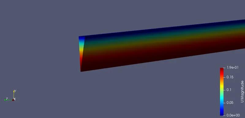
Velocity distribution Contour plot for different angles of the wedge :

The below contour plot is Velocity distribution at the outlet for 10 degrees wedge angle by considering the wedge BC.

:

The below contour plot is Velocity distribution at the outlet for 25 degrees wedge angle by considering the symmetry BC.

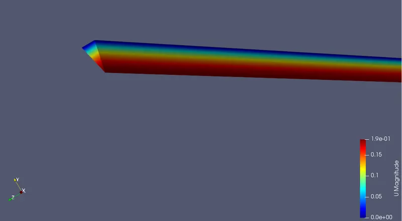
The below contour plot is Velocity distribution at the outlet for 45 degrees wedge angle by considering the symmetry BC.

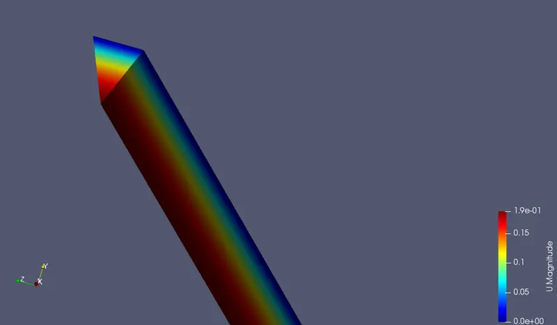
Validation of Results :

• Validation of Hydro-dynamic length with the numerical result :

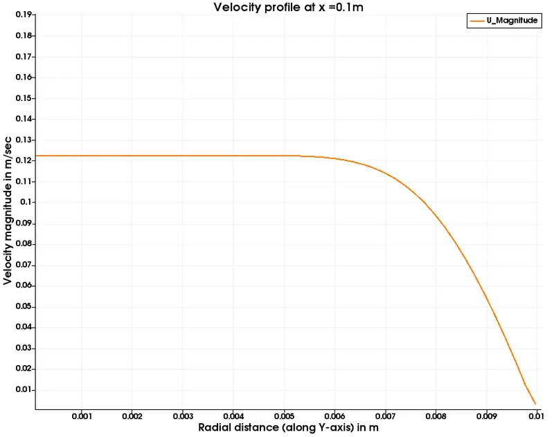
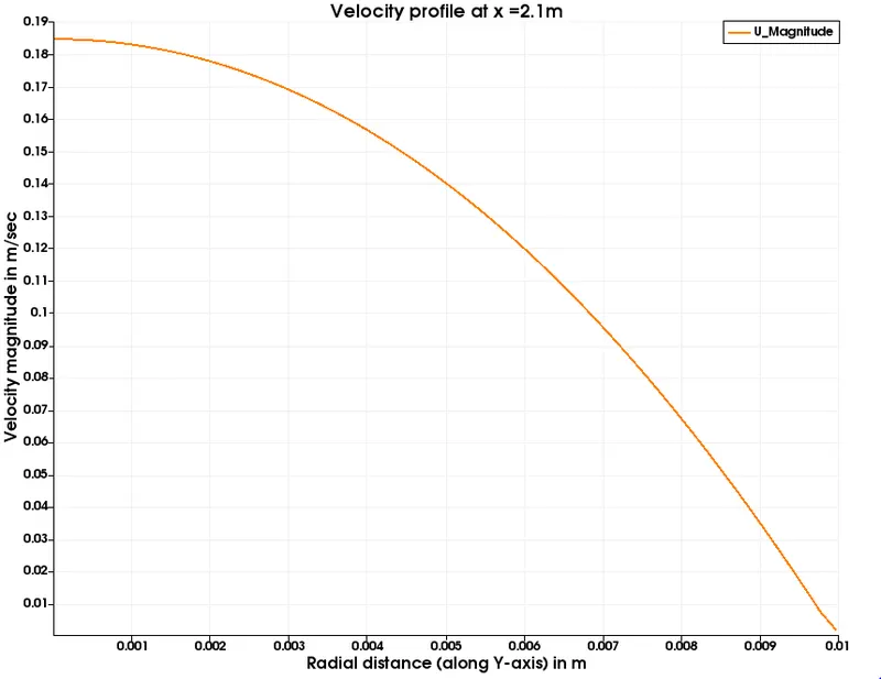
Now let us validate Hydro-dynamic length from Hagen poiseuille's flow with the numerical result.This is done by verifying the velocity profile ,which we calculate at different points along the flow direction .

Validation of Hydro-dynamic length with the numerical result for 10 degree wedge angle with wedge boundary condition :

Velocity profile at X= 0.1m :

It is the velocity profile when the fluid enters and cross the inlet of the pipe.

Velocity profile at X= 2.1m :

This is the velocity profile at the hydrodynamic length i.e, fully developed.

Velocity profile at X= 3.1m :

It is the velocity profile at the end of the pipe i.e, at the outlet.

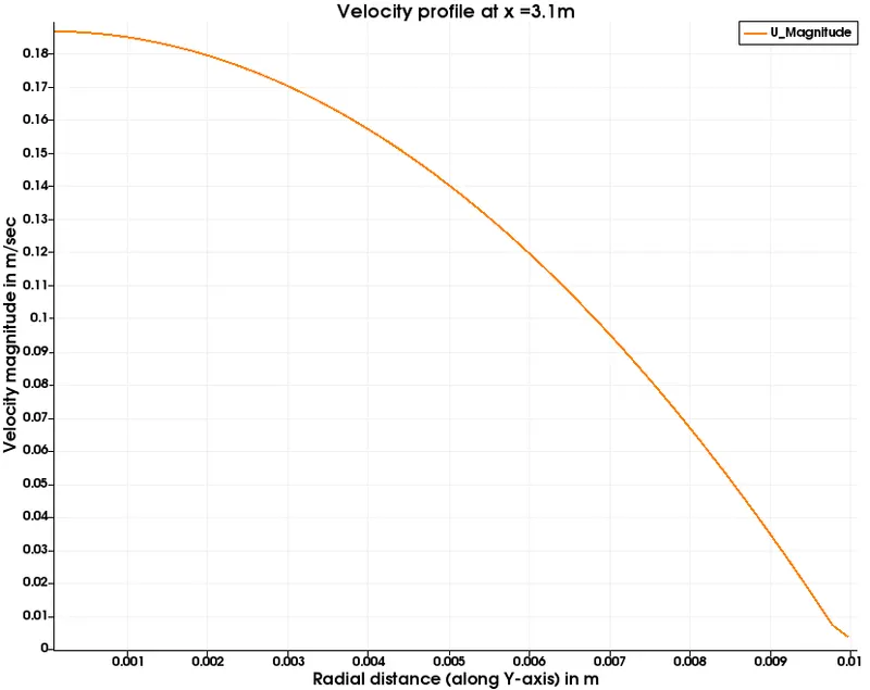
From the above plots we can observe that the velocity profile changes along the the flow direction continuously as the fluid progress through the pipe.As the fluid approaches the hydrodynamic length the maximum velocity goes on increasing and you can also observe that the velocity profile also becomes progressively more parabolic.When once the fluid reaches the hydrodynamic length i.e,at X =2.1, the flow becomes fully developed.And once it cross the hydrodynamic length the flow becomes fully parabolic and we can notice that the velocity profile is almost constant till it reaches the outlet.You can also observe from the plots that the maximum velocity is at the outlet i.e, 0.1867 m/sec.

Validation of Hydro-dynamic length with the numerical result for 10 degree wedge angle with symmetry boundary condition :

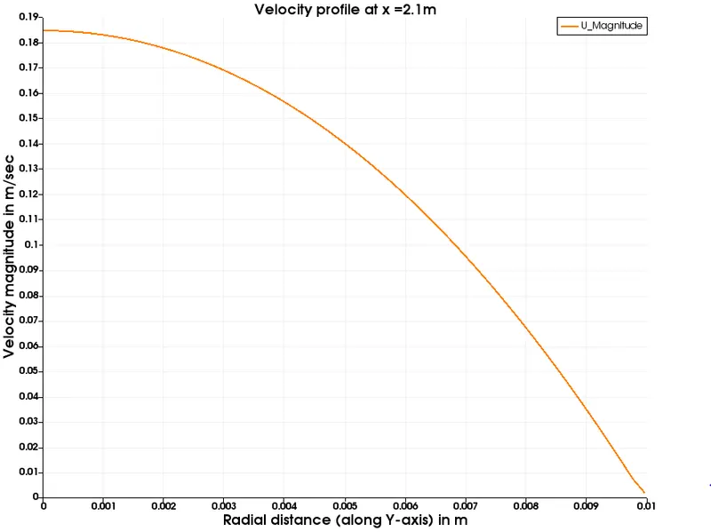
Velocity profile at X= 2.1m :

This is the velocity profile at the hydrodynamic length i.e, fully developed.

Velocity profile at X= 3.1m :

It is the velocity profile at the end of the pipe i.e, at the outlet.

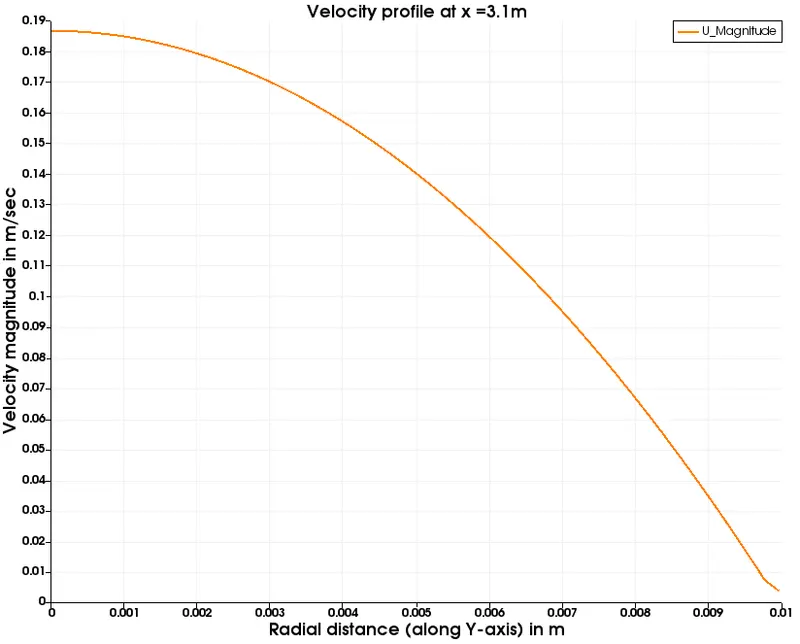
From the above plots we can observe that the velocity profile changes along the the flow direction continuously as the fluid progress through the pipe.As the fluid approaches the hydrodynamic length the maximum velocity goes on increasing and you can also observe that the velocity profile also becomes progressively more parabolic.When once the fluid reaches the hydrodynamic length i.e,at X =2.1, the flow becomes fully developed.And once it cross the hydrodynamic length the flow becomes fully parabolic and we can notice that the velocity profile is almost constant till it reaches the outlet.You can also observe from the plots that the maximum velocity is at the outlet i.e, 0.1867 m/sec,which is the same value which we got when we simulated with wedge BC .

The velocity profile which we calculate for different wedge angles will be almost same whether if you do with wedge BC or symmetry BC .The velocity profile will be almost constant till the outlet after flow cross the Hydro-dynamic length i.e, 2.1 m in all the cases.Hence from Hagen poiseuille's flow equations the Hydro-dynamic length is, 2.1 m which is equal to numerical result. Hence we have validated the Hydro-dynamic length from Hagen poiseuille's flow with the numerical result.

The thing that changes is the maximum velocity for every change in the angle the maximum velocity changes.Let's see more about in the validation of velocity.

• Validation of the fully developed flow velocity profile and maximum velocity with its analytical profile :

We validate the velocity profile of the fully developed flow with its analytical profile by comparing both the profiles, where we take the velocity profile data at the outlet from OpenFoam and take it in a spead sheet and transfer it to matlab and compare this profile with the analytical profile which is generated from the below formula in the matlab.

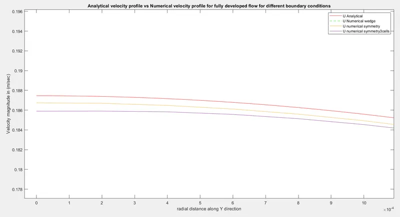
Matlab code for comparision velocity profiles for Analytical velocity profile vs Numerical velocity profile for fully developed flow for different boundary conditions :

clear all
close all
clc
r = linspace(0 ,0.01,1001);  % radial distance along Y direction
v_avg =0.093731193580742;     %average velocity
R= 0.01;                  %Maximum raidus of the pipe.                
for i =1:length(r)
U_analytical(i) = 2*v_avg*(1-(r(i)^2/R.^2)); %Analytical profile
end

%Numerical data imported from OpenFoam
velocity_1 = xlsread('1_vwedge.csv'); % velocity values whenwedge BC
 velocity_2 = xlsread('12_12symmetry.csv'); %velocity values when symmetry BC
 velocity_3 = xlsread('3_velocity3cells.csv');%velocity values when symmetry BC with 3 nodes in Z direction are considered

% seperated velocity data from the whole data
U_numerical_wedge =velocity_1(1:end,1); 
U_numerical_symmetry =velocity_2(1:end,1);
U_numerical_symmetry3 =velocity_3(1:end,1);

%plotting analytical velocity profile vs numerical velocity profile
 plot(r,U_analytical,'r',r,U_numerical_wedge,'g--',r,U_numerical_symmetry,r,U_numerical_symmetry3)
 legend('U Analytical','U Numerical wedge','U numerical symmetry','U numerical symmetry3cells')
 title('Analytical velocity profile vs Numerical velocity profile for fully developed flow for different boundary conditions')
 xlabel('radial distance along Y direction')
 ylabel('Velocity magnitude in (m/sec)')

The code is same for three different angles but the only thing to be changed is the filenames that contain the simulation data.

Velocity profile for 10 degree wedge angle :

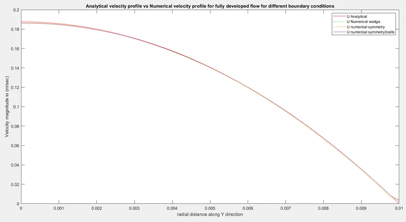
When you look into the above plot you can see that whatever the BC may be and also another case with symmetry boundary condtion by considering 3 cells in Z direction, in all these cases you can find out that they are in good ageement with analytical profile.But when you consider the closer view of these profiles the numerical solution that is obtained by wedge BC and symmetry BC with one cell in Z direction are equal and they are very nearest to the analytical profile,which are more accurate than the profile produced by symmetry boundary condtion in which 3 cells are considered in Z direction,which can be seen in the below plot.

Velocity profile for 25 degree wedge angle :

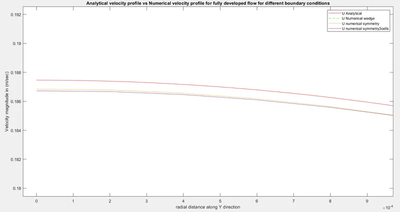
In the above plot we can observe that, the same thing happened in this case also, the numerical solution that is obtained by wedge BC and symmetry BC with one cell in Z direction are equal and they are very nearest to the analytical profile,which are more accurate than the profile produced by symmetry boundary condtion in which 3 cells are considered in Z direction

Velocity profile for 45 degree wedge angle :

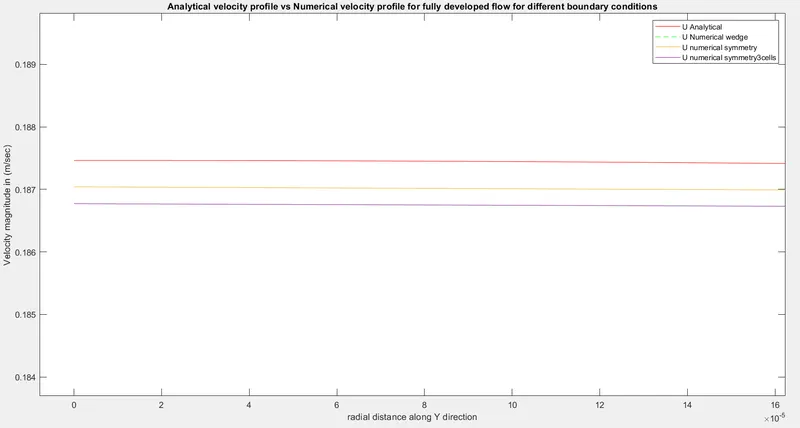
In the above plot we can observe that, the same thing happened in this case also, the numerical solution that is obtained by wedge BC and symmetry BC with one cell in Z direction are equal and they are very nearest to the analytical profile,which are more accurate than the profile produced by symmetry boundary condtion in which 3 cells are considered in Z direction.

Now let us compare the analytical profile with the numerical profile generated at different angles produced by symmetry BC to see at which wedge angle the velocity profile is captured close to the analytical solution.

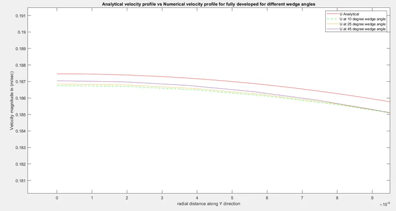
By seeing the above plot we can finally conclude that as the wedge angle is increasing we are getting close to the analytical solution i.e., The numerical velocity profile generated with wedge angle 45 degrees is very close to analytical solution.

Plots of pressure drop and wall shear stress for different wedge angle and boundary conditons :

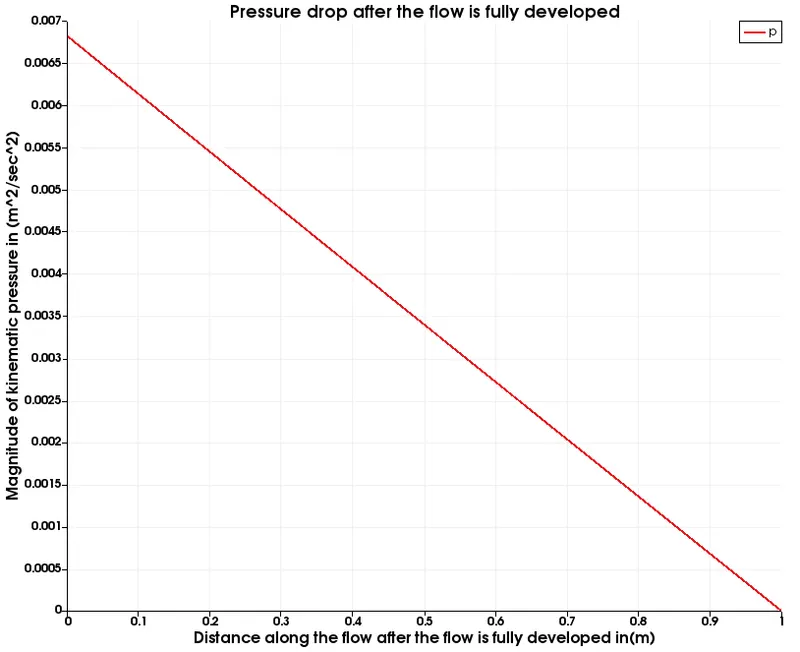
Kinematic pressure distribution plot for fully developed flow with wedge BC for wedge angle of 10 degrees :

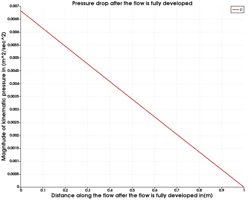
Kinematic pressure distribution plot for fully developed flow with symmetry BC for wedge angle of 10 degrees :

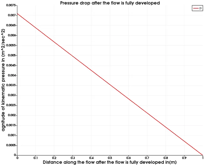
Kinematic pressure distribution plot for fully developed flow with wedge BC for wedge angle of 25 degrees :

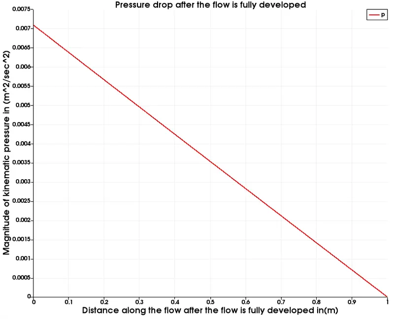
Kinematic pressure distribution plot for fully developed flow with symmetry BC for wedge angle of 25 degrees :

Kinematic pressure distribution plot for fully developed flow with wedge BC for wedge angle of 45 degrees :

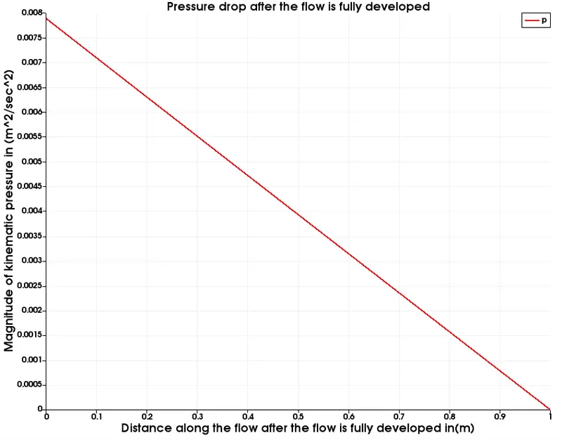
Kinematic pressure distribution plot for fully developed flow with symmetry BC for wedge angle of 45 degrees :

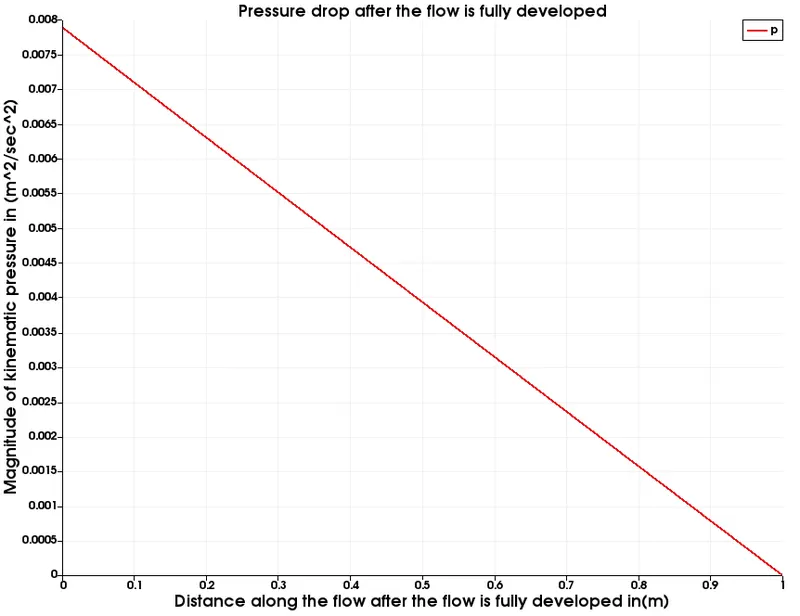
Wall shear stress distribution plot along the radial direction at X = 3.1 in for fully developed flow with wedge BC for wedge angle of 10 degrees :

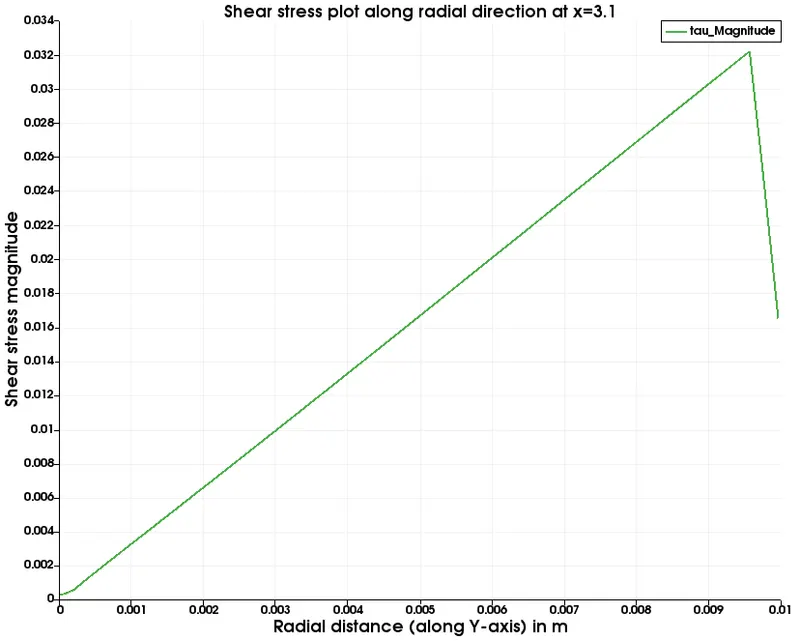
Wall shear stress distribution plot along the radial direction at X = 3.1 in for fully developed flow with symmetry BC for wedge angle of 10 degrees :

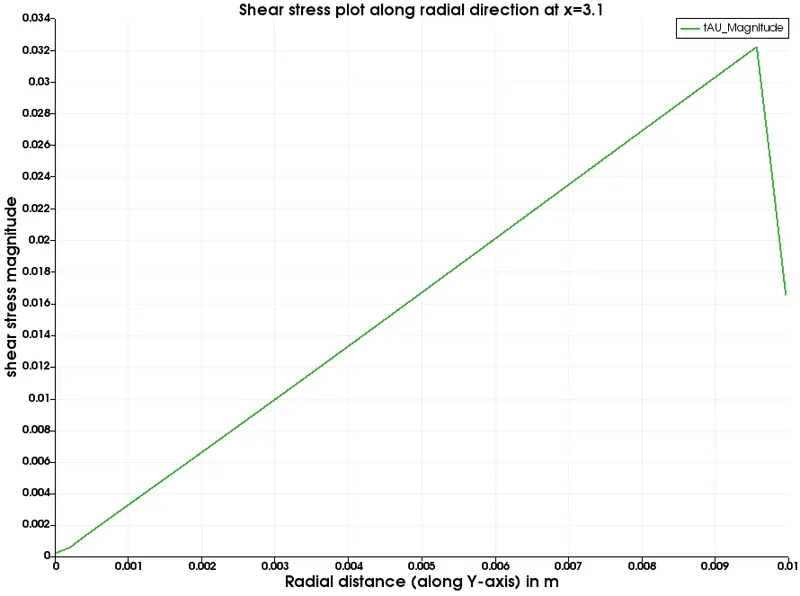
Wall shear stress distribution plot along the radial direction at X = 3.1 in for fully developed flow with wedge BC for wedge angle of 25 degrees :

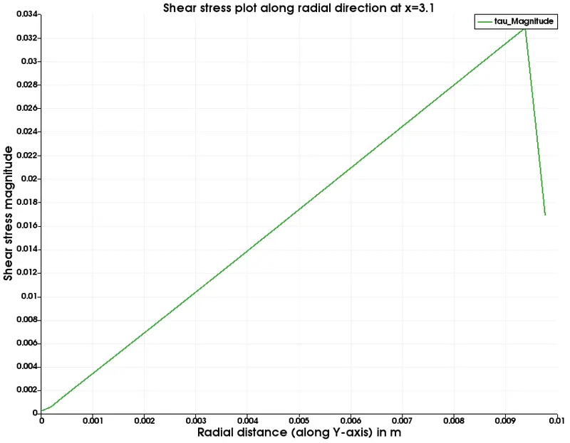
Wall shear stress distribution plot along the radial direction at X = 3.1 in for fully developed flow with symmetry BC for wedge angle of 25 degrees :

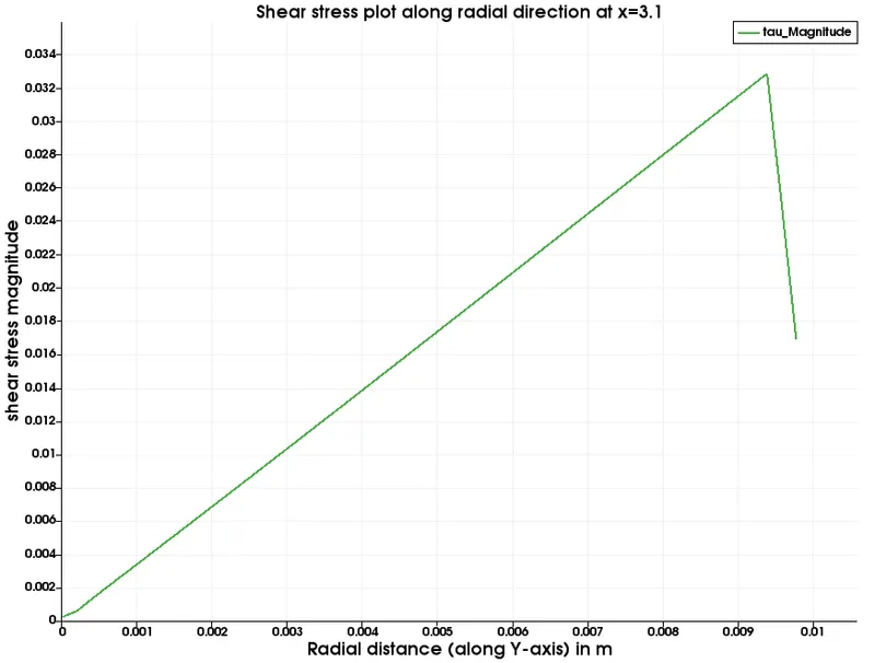
Wall shear stress distribution plot along the radial direction at X = 3.1 in for fully developed flow with wedge BC for wedge angle of 45 degrees :

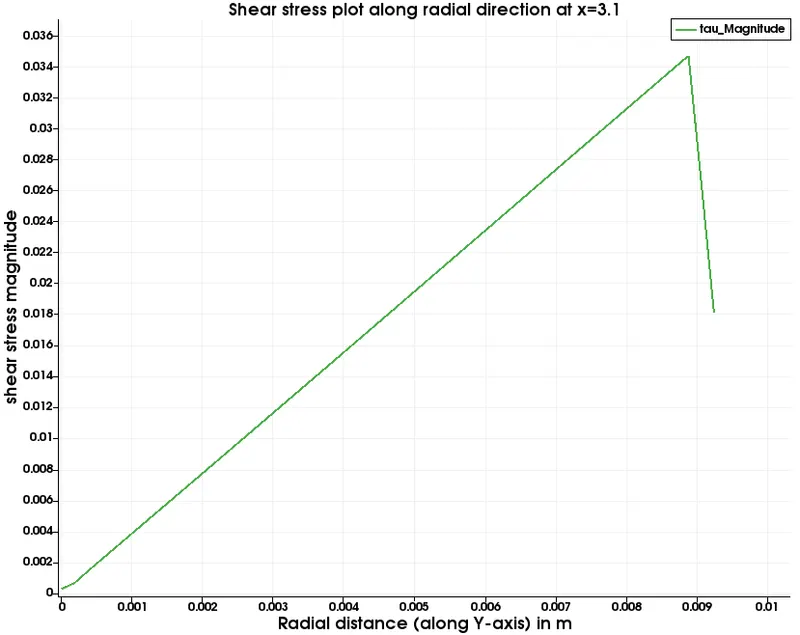
Wall shear stress distribution plot along the radial direction at X = 3.1 in for fully developed flow with symmetry BC for wedge angle of 45 degrees :

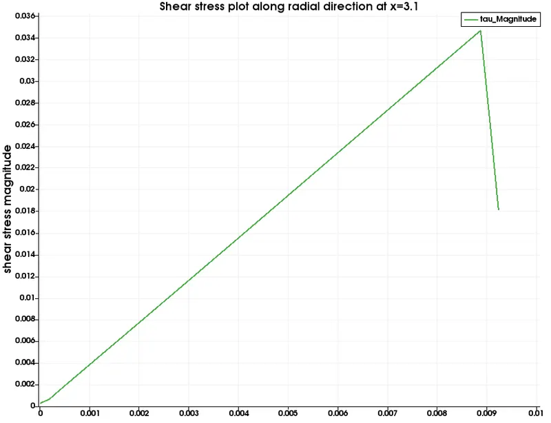
All of the above plots may look alike and very close to analytical but there is a small difference in the values.Let us tabulate the above data and validate the maximum velocity,pressure drop and wall shear stress with analytical solution.

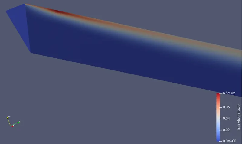
Comparision of wall shear stress contour plot at inlet of pipe and outlet for 25 degree wedge angle :

Wall shear stress contour plot at inlet of pipe :

Wall shear stress contour plot for fully developed flow (outlet of pipe) :

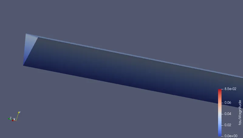
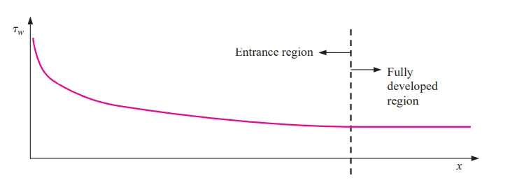
In the above two plots you can observe that the shear stress is maximum at the inlet of pipe but as the flow continues it's value getting dropped.But, at the outlet i.e., when the flow is fully developed the shear rate is constant there is not much change observed.

• Validation of Numerical result of maximum velocity ,pressure drop and shear stress simulated at different conditions for a fully developed flow with Hagen- Poiseuille's flow solution(Analytical solution) :
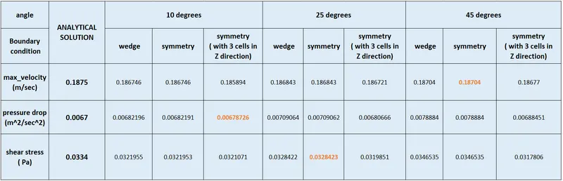
• The above table contains analytical values and simulated numerical data with different boundary and with different angles and also numerical data for symmetry BC with three nodes in Z direction.
• By observing the above table we can conclude that Almost all the values are in good agreement with analytical solution.
• We can also conclude that as the wedge angle is increasing we are getting close to the analytical value for maximum velocity. i.e., The numerical maximum velocity with wedge angle 45 degrees(0.18704 m/sec) is very close to analytical solution(0.1875m/sec).
• When comming to the pressure drop as the angle of wedge is increasing we are moving away from the analytical solution.So less wedge angle is desired to get the pressure drop more accurately.The values that are obtained with symmetry BC are far more closer to analytical solution.When we increase the no of rids in the Z-direction by choosing the symmetry boundary condition we are getting the pressure drop (0.00678726m^2/sec^2) even more close value to the analytical solution(0.0067m^2/sec^2).
• Finally comming to the shear stress almost all the values are very close to the analytical solution.As the wedge angle is increasing the maximum shear stress is increasing, but when we use the symmetry BC the values that are obtained are far more closer to analytical solution(0.0334pa).

Differences between wedge and symmetry conditions :

• When we use wedge boundary condition it calculates the value of flow variables by asssuming that our problem is 2-dimensional whereas when we use symmetry boundary condition it calculates the value of flow variables in 3-directions.
• When we solve the problem by giving 1 cell in in 3 rd direction there will not be much change whether we use symmetry or wedge boundary condition.When you increase the number of cells you can observe the change.So ,this is the reason why symmetry boundary condition captures more accurately.
• When we consider to solve using three cells it takes a lot of time to simulate the system as it is solving in 3-dimensional.When we use more than 3 cells by using symmetry BC you will see courant number crosses higher values and you will see an error, but when you use more than 1 cell you will see error by using wedge BC.This is also a advantage of symmetry BC.The reason why you get error is as you are considering in 3 dimensional ,so the courant number is also depend on dz ,where as more number of cells are increasing the dz will be too small.So,which causes courant number to increase and cause an error.How ever you can simulate it but decreasing the no of grids and time step size,but it will take much computational time and effort to simulate.
• Finally we can conclude that by using symmetry BC with more angle of wedge we will get very close to analytical velocity and by using symmetry BC with more number of cells in Z-direction and with less wedge angle we can capture the pressure distribution very well and close to analytical solution.