Objective :

In this challenge,

• We will perform a parametric study on the gate valve simulation by setting the opening from 10 % to 70%.
• Then we will obtain the mass flow rates at the outlet for each design point.
• Calculate the flow coefficient and flow factor for each opening .
• Then we will plot two graph for flow coefficient vs lift and flow factor vs lift.
• Then finally we discuss the results of the mass flow rate and flow coefficient for increasing lift.

Introduction :

• Here our objective is to simulate the flow through a gate valve by making the parametric study to analyze the flow rate at the outlet of the gate valve for different levels of gate valve disk.This gate disk valve is used to start or stop the fluid flow.
• The gate valve consists of a hand wheel and a spindle that is connected to the gate disk.The hand wheel and spindle together controls the level of gate disk.
• Let's start performing a parametric study on the gate valve simulation by setting the opening from 10 mm to 70 mm.

Solution procedure :

• To simulate the fluid flow and perform a parametric study on the gate valve simulation we follow the below procedure :

1)Geometry setup

2)Meshing

3) Problem setup

4)Solving

5)Post processing

Simulating the flow with the Steady case :

In the ANSYS work bench we first open the fluent module by drag and drop.The we follow the procedure we have mentioned above

1) Geometry setup :

• In fluent module we have to open spaceClaim and import the geometry.

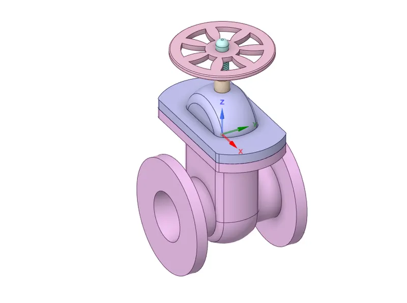
• Then as we need to parametrize the gate disk we need to follow the below steps,
• Step-1 : We need to pull the pipe’s outer solid surface before extracting the fluid volume.

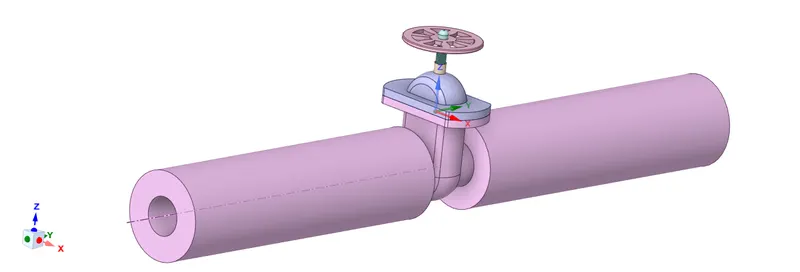
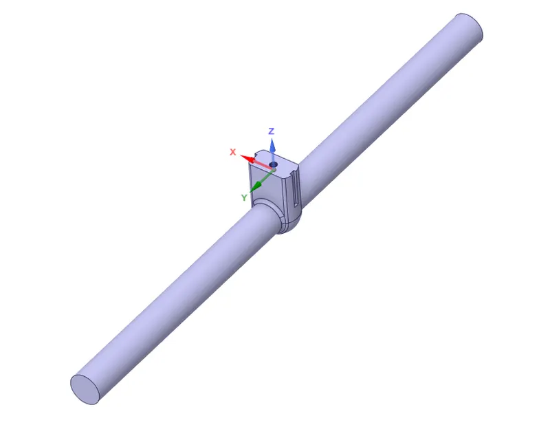
• Step-2 : Then we need to extract the fluid volume using 3 edges one is inlet and other outlet and the last one is top of the bottom case which is below the bonnet part.

To extract the fluid volume.For that we have to go to,

prepare -> volume extract -> select edge selection -> then select all the edges of inlet and outlet -> then click ok.fluid volume will be created .

• Step-3 : Suppress unwanted components.
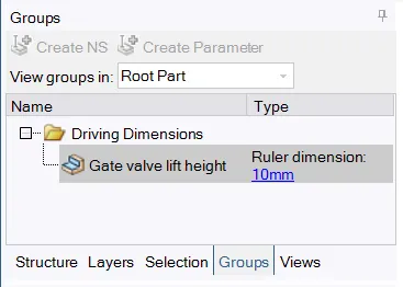
• Step-4 : Set the lift of the valve as a parameter.
• To set this we have to go to the Design tab and choose the Move option and further select Move Component and go on to select the Gate-Disc. Following which you will be able to see a Coordinate system appear on the gate disc, you can then proceed to move the gate disc towards the top of the spindle.
• Then to parametrize the same is to go to the Groups menu which is adjacent to the Structure menu; In the Group menu, you will able to see the Create Parameter button, which will be enabled only after you have moved the gate disc, click on the Create Parameter following which you will see a Group-1 appear in which you can edit the dimensions of the lift. This will have parameterized the Gate Disc lift, you confirm the same by checking your workbench.

• Step-5 : Update the extracted volume and update it as per the context so that the fluid volume will adapt automatically to the lift (change in solid geometry).We have to make sure bonnet is hidden while updating it within context.
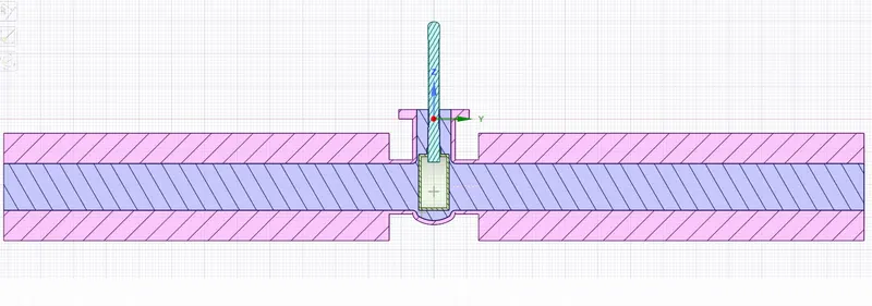
• The below image is the sectional view of domain with the fluid volume with gate vale lift of 10 mm.

• This completes the creation of geometry.Then we close the spaceClaim , the progress will be saved automatically.

2) Meshing :

• For meshing we open Meshing ,where we mesh our model so that we can use it to solve our model.
• In general it is always good to name the surfaces before meshing. So let us do that.
• We first select the entity by using the entity selection by using faces so that we can provide name for our entity selection.

steps : select the edge you want to name by using edge selection -> then press N -> name the selection.

• In the similar way we name our inlet and outlet.
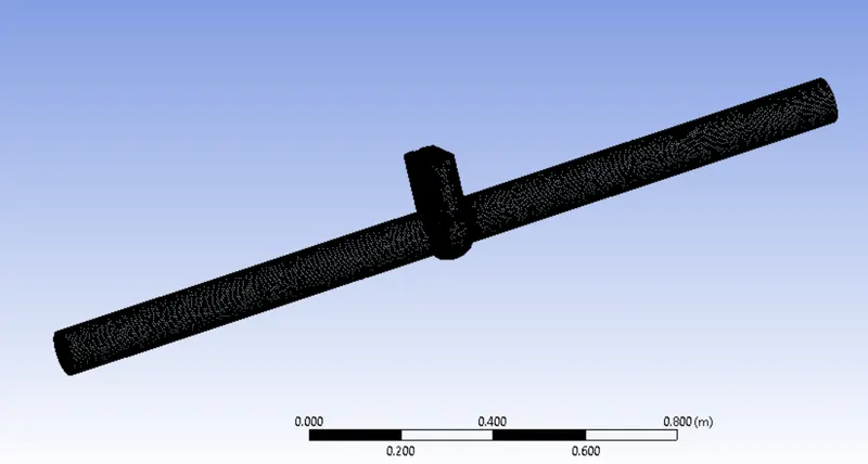
• Then next thing to do is to mesh.We click the mesh option in the side window and create our mesh by giving element size as 0.006 m.
• The below image is the final view of the mesh we have generated.

• Now we have to check the quality of the mesh.steps : mesh ->quality-> mesh metric-> Element quality
• Here our minimum quality is around 15 %,so we can move further for our solution setup.

3) Problem Setup :

• To set up our problem we open Fluent and setup inital conditions , boundary conditions material etc.,
• We first start with checking the mesh quality using perform mesh check under domain.If no error is seen in console window then we can proceed further.
• Then we move move to setting up physics where we select the solver ,viscous model ,initial and boundary conditions etc.,
• We use a steady state pressure based solver to solve our model.

Physics :

General :

Solver type : pressure based

time : steady state

velocity formulation : absolute

• We need to enable gravity by giving value for Z as -9.8 m/s^2 as gravity is acting in negative Y-direction.

models :

viscous model : k-epsilon Realizable model with Scalable wall functions

Material :

Fluid : Water-liquid

Zones :

Cell zone : In cell zones you will see fluid volume,it is of type fluid with material water-liquid .

Boundary conditions :We will basically give our boundary conditions here such as inlet and outlet conditions.

we give,

Inlet :

pressure inlet : 10 Pa

Outlet :

pressure outlet : gauge pressure = 0 pa

• Now if you check other BC they are just wall boundaries and interior we are not changing anything we are going to ignore them.
• Now we are almost ready to run the simulation ,but as the solution is being solved we want to moniter flow quantities while the solution is being generated.
  • Now we also want to moniter the mass flow rate and need to set it as output parameter to perform the parametric study.

• steps : Definitions -> New -> select the flux report -> select massflow rate-> in boundaries select outlet -> check report file and report plot -> and to parametrize the mass flow rate we need toselect/mark the output parameter -> then okay.

• In the same way you can also parametrize other quantities if needed.
• we also want to create pressure and velocity contour for this.But before that we have to initialize the domain.We use the Standard initialization from inlet , this provides a very good initial condition .
• Then we create a cut plane and plot the velocity and pressure contour on that plane.

For contour -> go to solutions tab -> graphics -> contour -> in contour of : select velocity under that velocity magnitude -> select the created plane and press save /display.

• Then you can see the initial values for velocity and pressure which is obtained by initialization which is not the final one.
• In the same way create the pressure contour plot also.
• we also want to create aminations so that as the solution is changing as the function of time we can see the physics behind it.
• Then we create animation so that we can see how these parameters are varying when problem is being solved.So that we can see the physics behind it.

For that,

steps : Activities -> solution animation -> select velocity contour,which we have created -> preview -> set the required view and use active -> and name it as velocity animation.

• In solution method we use Coupled .

4) Solving :

• Give iterations such that your solution is converged.
• Run the simulation until the steady state is reached.Lets run for 350 iterations , we can find the solution is converged.
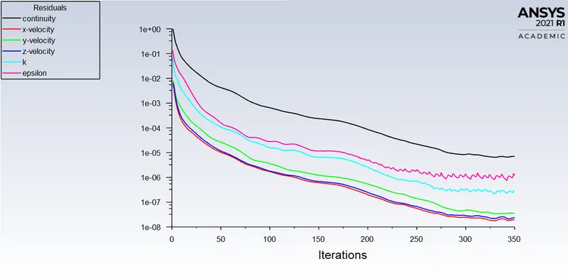
• Then we can see that in the residual plot that residuals dropping and reach a steady state after 300 iterations.
• Then let us post process the results.

5)Post processing :

Residuals plot :

• You can observe from the below plot the residuals has converged after 300 iterations.

Mass flow rate plot :

• To know the mass flow rate you can directly view in the console window or by opening the report definitions and clicking on compute.You will observe the value of mass flow rate as 0.14877521 kg/sec for a lift of 10 mm.

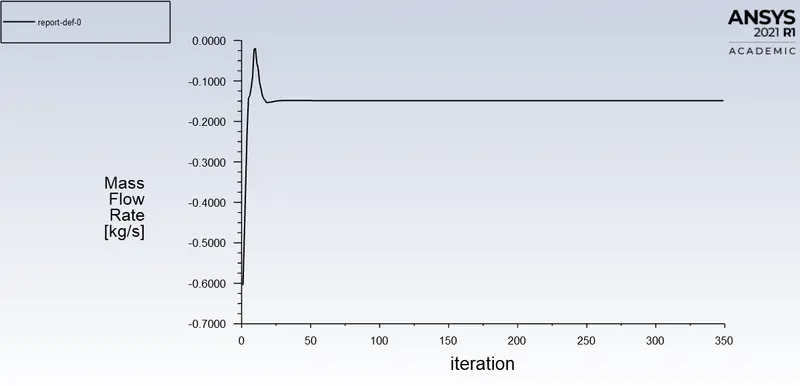
• You can see the negative value for the mass flow rate.This is because fluent assigns the negative sign for the mass flow rate for the fluid going out of the domain/volume and positive sign for the fluid entering the domain.

Velocity contour :

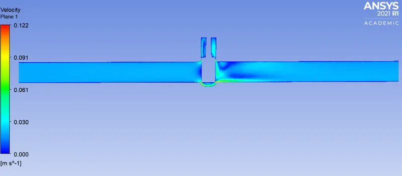
• In the below contour you can see the fluid velocity distribution in the pipe and near the gate valve.

Pressure contour :

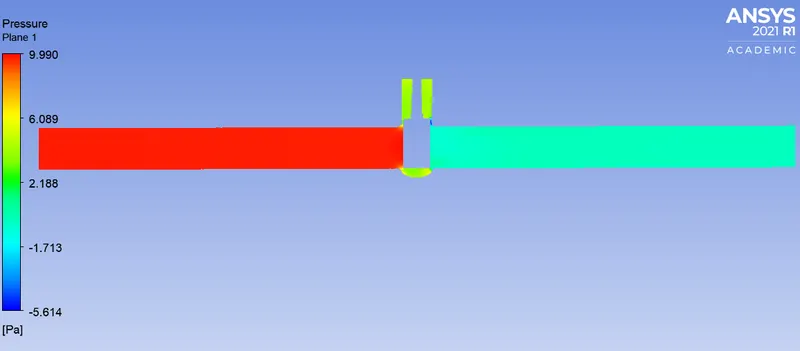
• In the below contour you can see the fluid pressure distribution in the pipe and near the gate valve.

Parametric study on the gate valve :

• Now if you close the fluent and go back to workbench you will observe a new option has added ie., parameters.
• If you double click on it you will find a new tab is opened as shown in the below image.

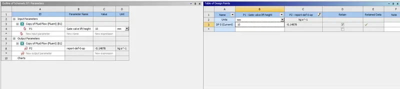
• In the left side tab you will find the input and output parameters and in the right side tab you will see a table consisting of design point with input gate lift value and output mass flow rate.
• There you can also obserrve a empty row to create new design point.There we give a input for the new gate lift value from 20 ,30 ... upto 70 mm.
• To view the updated geometry ,meshing ,solution data ,animations ,contours etc. of newly created design point you need to click on the retain data.
• Now wee need to update all the design point by clicking on the update all design points.
• After updating the design points you will observe the values of mass flow rate in the mass flow rate output column for all the created design points as shown in the below image.

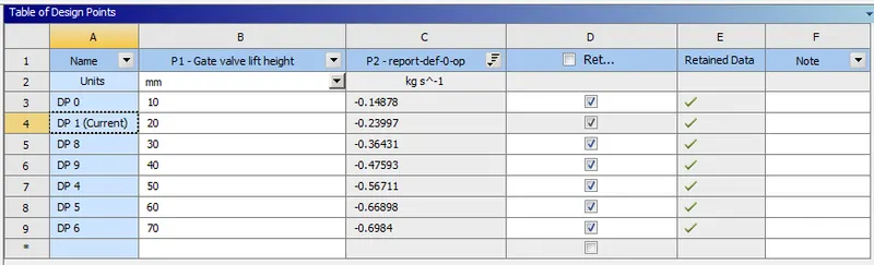
• Then after that you can see the individual solution date by right click on the name of design point and selecting set as current.Then you can go to workbench and view the result of the required design point.
• Now let us plot the velocity contour and mass flow rate plot for all the cases.

Mass flow rate plot and Velocity contour for a lift of 20 mm :

Mass flow rate plot :

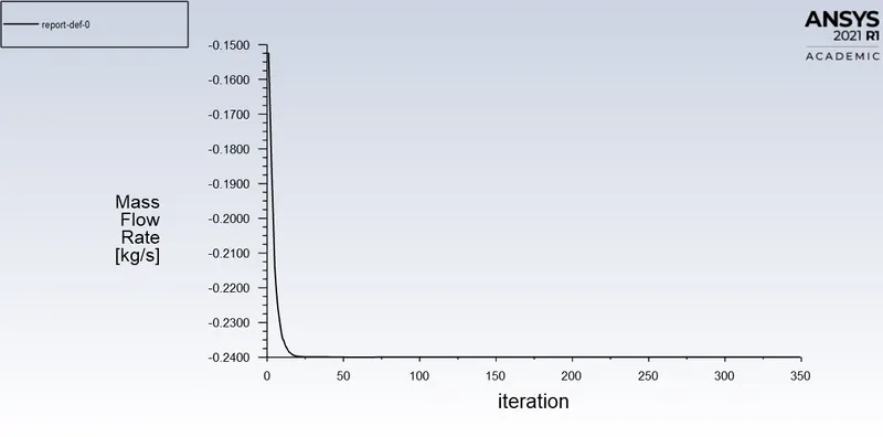
• To know the mass flow rate you can directly view in the console window or by opening the report definitions and clicking on compute.You will observe the value of mass flow rate as 0.23996638 kg/sec.

Velocity contour :

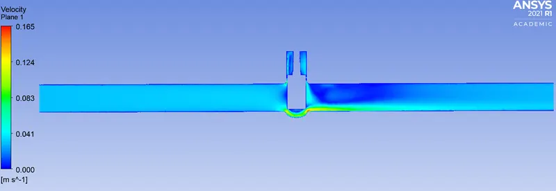
• In the below contour you can see the fluid velocity distribution in the pipe and near the gate valve.

Mass flow rate plot and Velocity contour for a lift of 30 mm :

Mass flow rate plot :

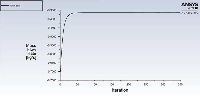
• To know the mass flow rate you can directly view in the console window or by opening the report definitions and clicking on compute.You will observe the value of mass flow rate as 0.3643145 kg/sec.

Velocity contour :

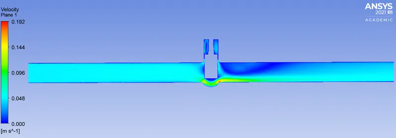
• In the below contour you can see the fluid velocity distribution in the pipe and near the gate valve.

Mass flow rate plot and Velocity contour for a lift of 40 mm :

Mass flow rate plot :

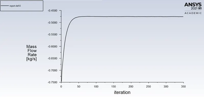
• To know the mass flow rate you can directly view in the console window or by opening the report definitions and clicking on compute.You will observe the value of mass flow rate as 0.47592567 kg/sec.

Velocity contour :

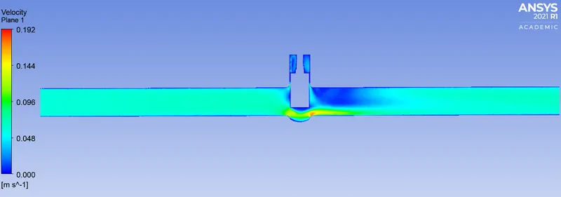
• In the below contour you can see the fluid velocity distribution in the pipe and near the gate valve.

Mass flow rate plot and Velocity contour for a lift of 50 mm :

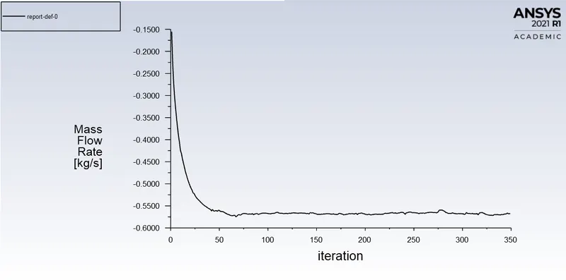
• To know the mass flow rate you can directly view in the console window or by opening the report definitions and clicking on compute.You will observe the value of mass flow rate as 0.56711282 kg/sec.

Velocity contour :

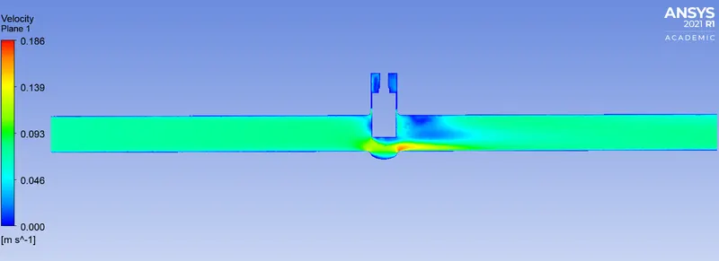
• In the below contour you can see the fluid velocity distribution in the pipe and near the gate valve.

Mass flow rate plot and Velocity contour for a lift of 60 mm :

Mass flow rate plot :

• To know the mass flow rate you can directly view in the console window or by opening the report definitions and clicking on compute.You will observe the value of mass flow rate as 0.66897892 kg/sec.

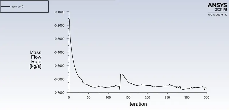
Velocity contour :

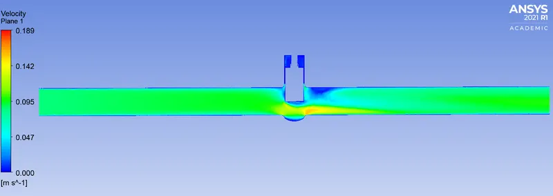
• In the below contour you can see the fluid velocity distribution in the pipe and near the gate valve.

Mass flow rate plot and Velocity contour for a lift of 70 mm :

Mass flow rate plot :

• To know the mass flow rate you can directly view in the console window or by opening the report definitions and clicking on compute.You will observe the value of mass flow rate as 0.69839513 kg/sec.

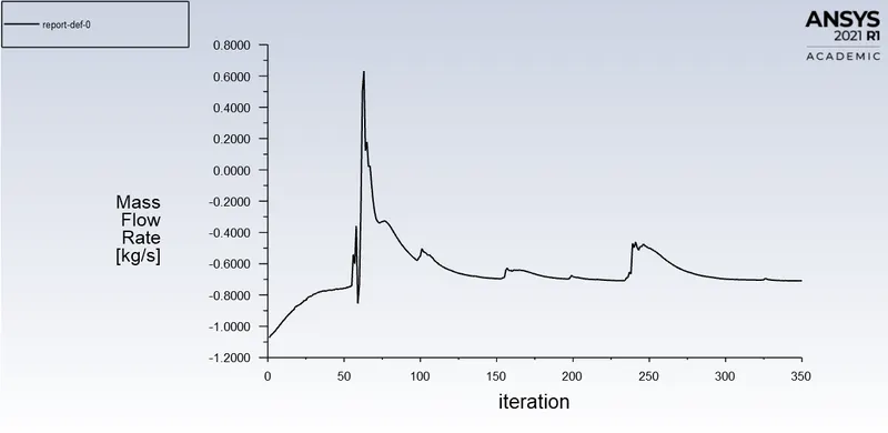
Velocity contour :

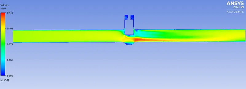
• In the below contour you can see the fluid velocity distribution in the pipe and near the gate valve.

Calculation of the flow coefficient and flow factor for each opening :

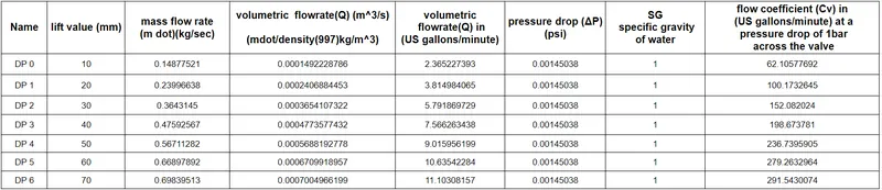
Flow coefficient :

• The flow coefficient of a device is a relative measure of its efficiency at allowing fluid flow. It describes the relationship between the pressure drop across an orifice valve or other assembly and the corresponding flow rate.
• Mathematically the flow coefficient C_v (or flow-capacity rating of valve) can be expressed as :

where:

Q is the rate of flow (expressed in US gallons per minute),

SG is the specific gravity of the fluid (for water = 1),

ΔP is the pressure drop across the valve (expressed in psi).

• In more practical terms, the flow coefficient C_v is the volume (in US gallons) of water at 60 °F that will flow per minute through a valve with a pressure drop of 1 psi across the valve.
• The use of the flow coefficient offers a standard method of comparing valve capacities and sizing valves for specific applications that is widely accepted by industry. The general definition of the flow coefficient can be expanded into equations modeling the flow of liquids, gases and steam using the discharge coefficient.

Calculation of the flow coefficient :

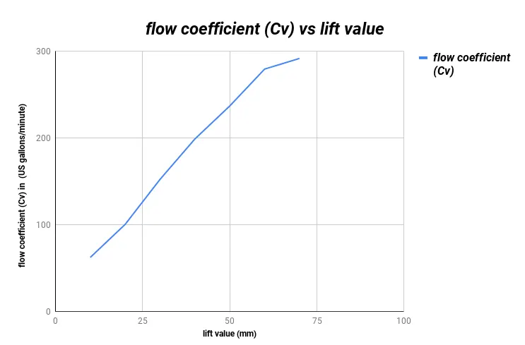
Plot showing flow coefficient vs lift of gate valve :

Flow factor :

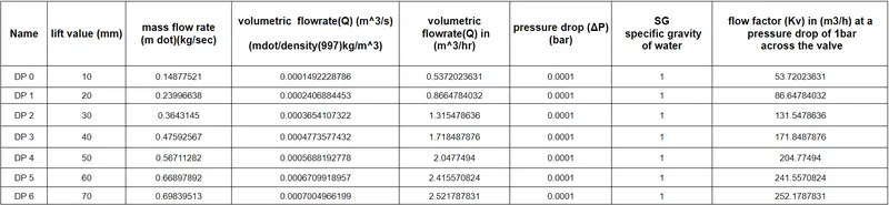
• The k_v factor of a valve indicates "The water flow in m³/h, at a pressure drop across the valve of 1 bar when the valve is completely open. The complete definition also says that the flow medium must have a specific gravity of 1000 kg/m³ and a kinematic viscosity of 10⁻⁶ m²/s. e.g. water.
• The metric equivalent flow factor (K_v; commonly used everywhere else in the world with the exception of the United States) is calculated using metric units :

where ,

K_v is the flow factor (expressed in m^3.h-1

Q is the flowrate (expressed in cubic metres per hour m^ 3. h,

SG is the specific gravity of the fluid (for water = 1),

∆P is the differential pressure across the device (expressed in [bar]).

• K_v can be calculated from C_v using the equation:

Calculation of the flow factor :

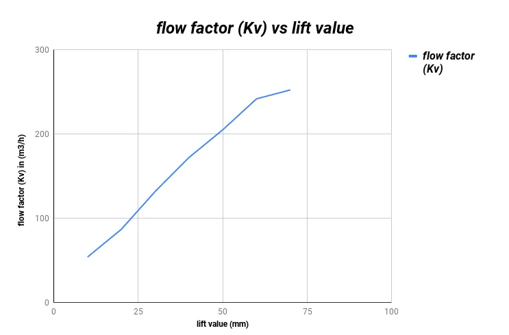
Plot showing flow factor vs lift of gate valve :

Comparision of results of the mass flow rate and flow coefficient for increasing lift :

• If you look at the results it is same as we expect with the increasing lift there is an increase in the mass flow rate .
• When you look at the flow factor and flow coefficient they have they have the same flow rate units as mass flow rate but with different units and flow coefficient and flow factor are flow passing gallons per minute and m^3 per hour respectively through a valve with a pressure drop of 1 psi and 1 bar across the valve respectively.
• If you see the formula , Cv =0.865 Kv our results also exactly same , following the formula.
• So we can easily guess and see in the results that as gate valve lift value is increasing we can see there is an increase in the value of flow coefficient and flow factor.

Animations :

• Velocity distribution animation of a gate valve simulation for a lift of 30 mm(Steady state).

• Velocity distribution animation of a gate valve simulation for a lift of 40 mm(Steady state).