Week 2 - Flow over a Cylinder.

Objective :

In this challenge we simulate the flow over a cylinder and explain the phenomenon of Karman vortex street,

1. We will simulate the flow over cylinder with the steady and unsteady case. In both approaches, we show that the flow has converged and calculate the Strouhal Number for Re= 100.
2. Plots of the coefficient of drag and lift and plots to show vortex shedding behind the cylinder.
3. Calculate the coefficient of drag and lift over a cylinder by setting the Reynolds number to 10,100,1000,10000 & 100000 by using steady state solver.
4. Then finally, we discuss the effect of Reynolds number on the coefficient of drag.

Introduction :

• External flows in general can be classified as flows over immersed bodies where flow features (such as boundary layers) around the body can develop freely without constraints of adjacent surfaces:
  ‐ Airflow over aircraft and ground vehicles
  ‐ Water flow over a submersible vessel
  ‐ Flying baseballs, footballs and golf balls
• One of the most important areas of interest in studying external flows are fluid forces acting on the body, as they define the dynamics of an object traveling through a fluid.
• Unlike internal flows which could be solved analytically for the entire range of laminar 𝑅𝑒, analytical solutions to flows over even simple shapes are only possible for very low Reynolds numbers 𝑅𝑒~1 which are of little interest in practical applications.
• Even at modest laminar regime numbers 𝑅𝑒~10, external flows start developing separation regions and wakes which cannot be described analytically.
• The boundary layer theory for laminar and turbulent flows provided us with relations and correlations which can clarify some, but not all, characteristics of external flows.
• An external flow is, indeed, a challenging problem even in present-day fluid dynamics.
• To highlight challenges in predicting external flows, let’s consider a flow over a very simple cylindrical shape.Even though the shape is simple, the flow is not!.
• At 𝑅𝑒 ∝ 10 the flow starts separating and developing a stationary wake.
• As the Reynolds number increases, the wake becomes unsteady and evolves into periodically shed vortical structures.
• Such unsteady evolution of the wake leads to time-fluctuating fluid forces whose prediction becomes challenging even in the laminar regime.
• The flow around a two-dimensional circular cylinder is case that has been used both as a validation case and as a legitimate research case. At very low Reynolds numbers, the flow is steady and symmetrical. As the Reynolds number is increased, asymmetries and time-dependence develop, eventually resulting the famous Von Karmann vortex street, and then on to turbulence.
• The problem geometry is two-dimensional and there is some variation in the details (both geometry and boundary conditions) that can be used. A typical geometry is shown below (not to scale).This problem has been solved as both a laminar flow and a turbulent flow. The DNS, LES, and the transitional cases are still considered a research cases. Many different numerical techniques have been used to solve this problem, but one usual comparison is the the resulting Strouhal frequency.

Boundary Layer Separation :

• In general, wall-bounded flows are subject to pressure variations due to surface curvature or an external forcing.
• When the freestream pressure increases in the direction of flow, it is known as an adverse pressure gradient.
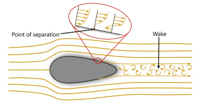
• Adverse pressure gradients cause the flow to slow down. When the velocity gradient at the wall approaches zero, the flow will lift off the surface, diverting the streamlines away from the wall. This process is known as separation.
• When a boundary layer becomes separated, the boundary layer equations are no longer valid. However, we can predict the point of separation by monitoring the velocity gradient (or shear stress) at the wall in our solution and noting where it becomes close to zero.
• The pressure field in the fluid flow past an object is nonuniform. When the pressure gradient is nonzero, the velocity profile is affected .
• Separation of boundary layers in general occurs when the velocity of the boundary layer “struggling” against an adverse pressure gradient becomes nearly zero, i.e, pressure increases as the wall fade away this pushes the fluid back .If the momentum of fluid is insufficient the fluid reverses its direction and seperates from the wall.
• The separation point is defined as a location between forward and inverse flow where the wall shear stress is zero.
• The thickness of the boundary layer abruptly increases at the separation point, and the layer is forced off the surface by the reversed flow near the wall.
• Detached flow takes the form of vortical structures, which can be laminar or turbulent depending on the flow regimes.

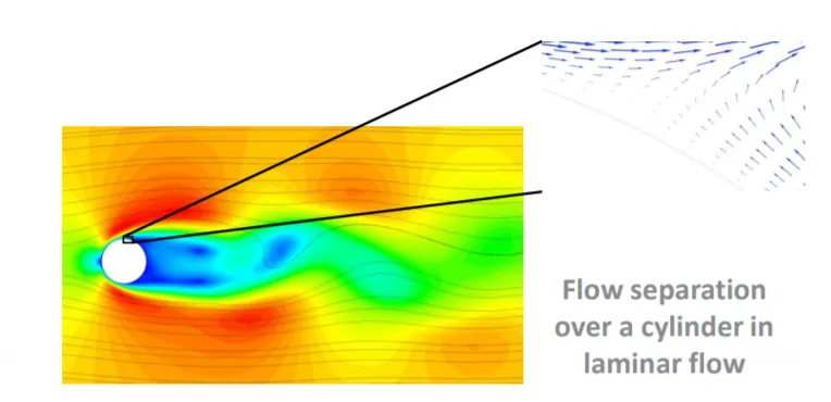
• Boundary layer separation can, under a certain range of Reynolds numbers, generate a repeating pattern of vortices. This trail of vorticies is called the Karman vortex street.
• Vortex shedding in the Karman street locks into a self-sustained periodic pattern at a singular frequency (expressed in terms of non-dimensional Strouhal number) as

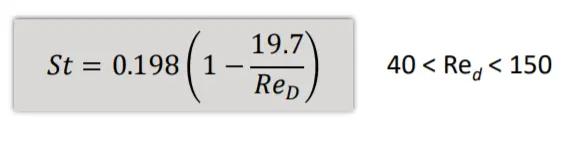
• Karman vortex shedding can be observed in nature and in man-made devices.Periodic vortex shedding results in periodic fluid forces on the surface of the object.
• At higher Reynolds numbers periodic vortex street transitions into a turbulent wake, but identifiable periodicity in fluctuations of separating boundary layers remains, and an identifiable tonal frequency can be identified up to 𝑅𝑒~10^5.
• Forces induced on object’s surface by periodic separation fluctuations have two distinct side effects as they:
  ‐ generate acoustic (sound) waves in a compressible fluid (think of noise emitted by a rapidly spun thin rope)
  ‐ can become culprits of resonant effects in the structure of the object when their frequency coincides with anatural frequency of the structure.
• Now let us simulate the flow over cylinder to simuate the Von Karman vortex street.

Solution procedure :

• We will simulate the flow over cylinder with the steady and unsteady case. In both approaches, we show that the flow has converged and calculate the Strouhal Number for Re= 100.
• Then for solving we follow the below procedure :

1)Creation of geometry

2)Meshing

3) Problem setup

4)Solving

5)Post processing

• Then while simulating the model, in both approaches we plot the coefficient of drag and lift and plot to show vortex shedding behind the cylinder and then finally we show that the flow has converged .Then we will post process the results and take the required results to find Strouhal number and compare them with analytical solution.
• Then we calculate the coefficient of drag and lift over a cylinder by setting the Reynolds number to 10,100,1000,10000 & 100000 by using steady state solver.
• Then finally, we discuss the effect of Reynolds number on the coefficient of drag.

Simulating the flow with the Steady case :

In the ANSYS work bench we first open the fluent module by drag and drop.The we follow the procedure we have mentioned above

1) Creation of geometry :

• In fluent module we have to open spaceClaim.
• Then firstly we draw a cylinder of diameter 2m.
• Then we create a computational domain around the cylinder with dimensions in front 10D =20m and back side of cylinder 20D =40m aand a with of 5D= 10m on both sides from the center of cylinder.
• We draw these by using construction lines then after creating the required domain we convert the created domain in to surface by using the pull tool.
• Then we select the inside cylinder and construction lines and delete them.

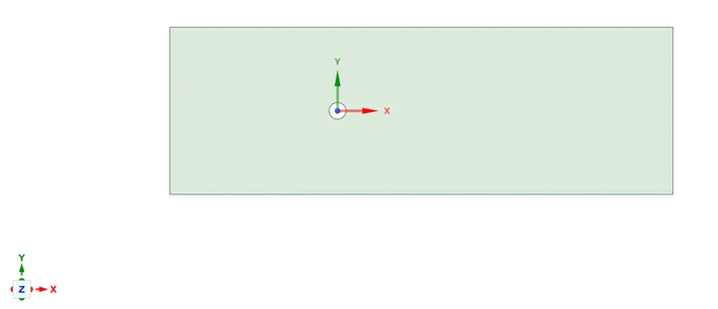
• This completes the creation of geometry.Then we close the spaceClaim ,the progress will be saved automatically.

2) Meshing :

• For meshing we open Meshing,where we mesh our model so that we can use it to solve our model.
• We first select the entity by using the entity selection by using faces so that we can provide name for our entity selection.

steps : select the edge you want to name by using edge selection -> then press N -> name the selection.

• In the similar way we name our inlet,outlet,symmetry walls and cylinder wall.
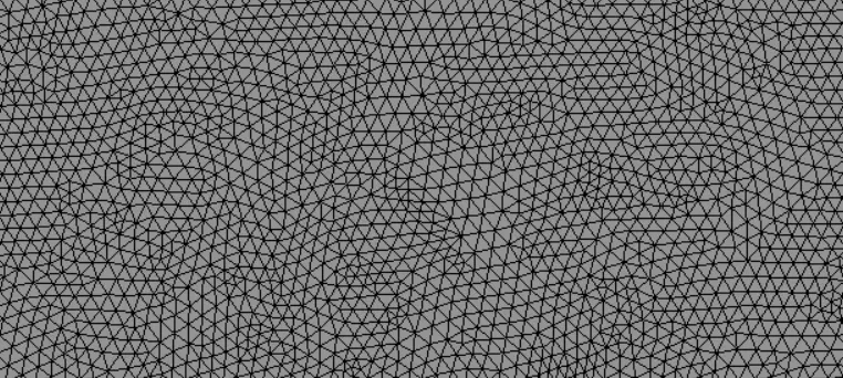
• Then next thing to do is to mesh.We click the mesh option in the side window and create our base line mesh.We then refine mesh.Let's mesh the geometry with 0.1m.Once the mesh has done we need to see what are the things we have to refine.Let us refine one by one .

a) Method (All triangle method) :

• For our geometry we need tria elements to be more to get the geometry in a better way.To create this we need to select method by right clicking on mesh option and then select the method to triangle,to make the mesh a tria dominant.

b) Sizing :

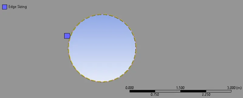
• To get a perfect cylinder shape(circle as it is 2D) sufficient for our case we need to increase the no. of divisions of the circle for that here we select the sizing.
• In sizing,In type we select number of divisions and we give 36,that's sufficient fo our case .

c) Inflation :

• Inflation layer helps us to create a body fitted mesh.It means it creates a layer of mesh same as the geometry around the orginal cylinder .
• Since the flow around the cylinder is very important we need to take that region and create inflation layers so that flow is captured exactly.
• Here we use first layer thickness 0.01 mm and numbers of layers = 6.The layer size inceases from layer to layer depending upon the growth ratio we give.Here we growth ratio as 1.2.

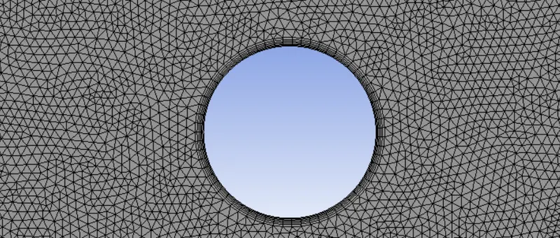
• By this we have completed the meshing process then we update or generte the mesh again.

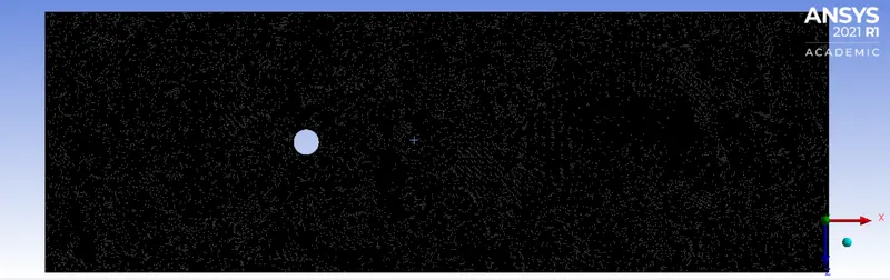
• Now we have to check the quality of the mesh.
• steps : mesh ->quality-> mesh metric-> Element quality

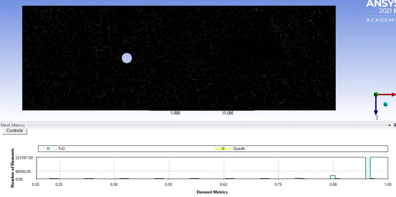
• Here our minimum quality is around 23% ,so we can move further for our solution setup.

3) Problem Setup :

• To set up our problem we open Fluent and setup inital conditions , boundary conditions material etc.,
• We first start with checking the mesh quality using perform mesh check under domain.If no error is seen in console window then we can proceed further.
• Then we move move to setting up physics where we select the solver ,viscous model ,initial and boundary conditions etc.,
• We use a steady state pressure based solver to solve our model.

Physics :

General :

Solver type : pressure based

time : steady state

velocity formulation : absolute

• Then we select the viscous model as laminar since the reynolds number is very small the flow will be laminar.

models :

viscous model : laminar

Material :

• Here the way we are going to control our Reynolds number is by modifying the dynamic viscosity of our working fluid.
• The way we do this is in materials we the air and we rename it we change the value of denisty and viscosity of our fluid so that the Reynolds number is equal to 100.

Density = 1 kg/m^3

Viscosity = 0.02 kg/m.s

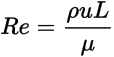
• Here as our characteristic length is 2 m and we give the inlet velocity value as 1 m/sec we get the Reynolds number =100 .
• This is the condition where we can can surely see the vortex shedding around the cylinder(Karman vortex street).

Zones :

Cell zone : you will see our volume zone which is basically our internal volume basically mesh, and it is of type fluid.We change the material here, which we have just created.

Boundary conditions :We will basically give our boundary conditions here such as inlet velocity and outlet conditions.

we give,

Inlet -x :

velocity : 1 m/sec

Outlet :

pressure outlet : gauge pressure = 0 pa

Cylinder Wall :

wall : No slip

• Now we are almost ready to run the simulation ,but as the solution is being solved we want to moniter different flow quantities while the solution is being generated ,we use definitions for this.
• We want to see vortex average at a point,for that we need a moniter point ,we have to create a point.

steps : In results -> create -> point(which we want to create at a distance of 4D from the origin(x = 8 m Y = 0 m from origin)) -> give values -> name it as moniter poin t and click create.

• Now we want to create vortex average at a point .

steps : Definitions -> New -> select the surface report ->vertex average -> field variable : velocity -> velocity magnitude -> under surface -> select the moniter point which we have just created -> check

report file and report plot ->then okay.

• Now we also want to moniter the lift and drag coefficient plot while the solution is being run.Create lift and drag coeffcients plots.

steps : Definitions -> New -> select the force report -> drag -> select cylinder wall under zones -> check report file and report plot -> then okay.

• In the same way create a plot for lift coefficient also.
• we also want to create aminations so that as the solution is changing as the function of time we can see the physics behind it.
• Pressure and velocity contours :
• We want to see the pressure and velocity contour as the solution is being generated. For that we have to initialize the domain first.
• We use the standard initialization from the inlet.Thento create contour we follow below steps ,

For contour -> go to solutions tab -> graphics -> contour -> in contour of : select velocity under that velocity magnitude -> select all the surfaces and press save /display.

• Then you can see the initial values for velcity which is obtained by initialization which is not the final one.
• In the same way create the pressure contour plot also.
• Then we create animation so that we can see how these parameters are varying when problem is being solved.
• In solution method we use SIMPLE .
• In residuals we have continuity , X- velocity ,Y- velocity.We uncheck convergence because we want to see solution till the number of iterations we input ,so that the solving doesn't stop when it gets converged.

4) Solving :

• Give iterations such that your solution is converged.Not only residuals but also some physical parameters which are important.In our case that could be the velocity in the moniter point location.
• Run the simulation until the steady state is reached.Lets run for 3000 iterations ,we can find the solution is converged.
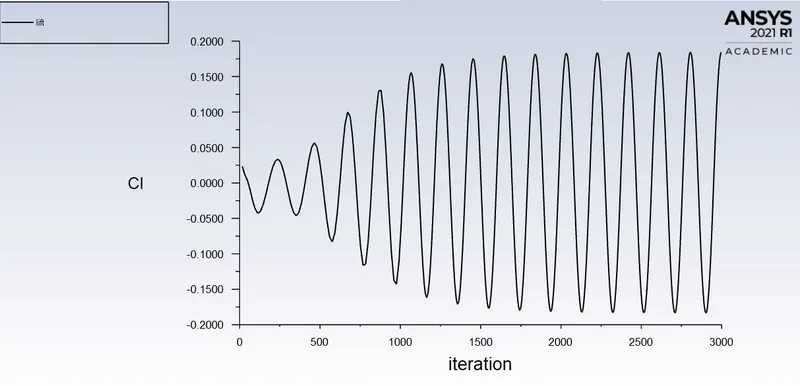
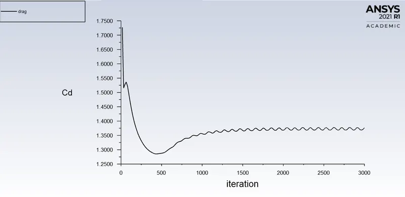
• Once it cross 500 iterations you will see the vortex shedding and after 1700 iterations you can observe all the plots has obtained steady state.Then post process the results.
• Then we can see that in the residual plot we see residuals dropping and reach a steady state after 175 iterations.

5)Post processing :

Residuals plot :

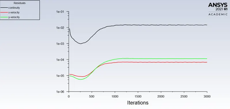
• You can observe from the below plot the residuals has converged after 1000 iterations.

Vortex average plot :

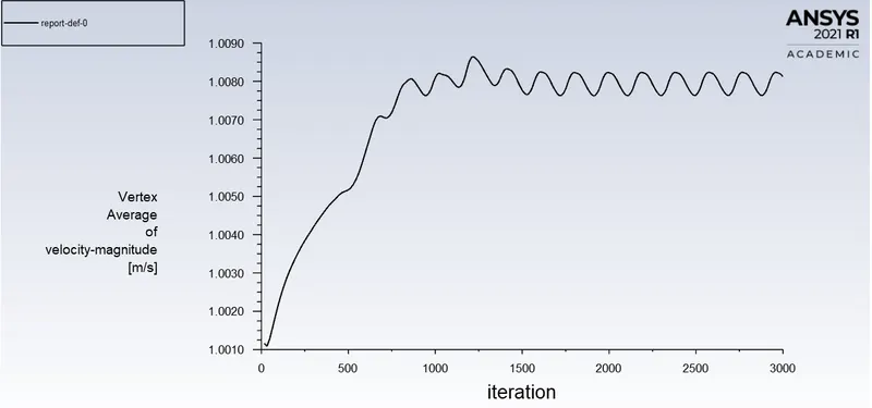
• You can observe from the below plot that vertex average has reached the steady state as it follows the same pattern after 1700 iterations.So we can conclude that the flow has converged.

Lift plot :

• You can observe from the below plot that lift coefficient has reached the steady state as it follows the same pattern after 1700 iterations.So we can conclude that the flow has converged.

Drag plot :

• You can observe from the below plot that drag coefficient has reached the steady state as it follows the same pattern after 1600 iterations.So we can conclude that the flow has converged.

Velocity contour :

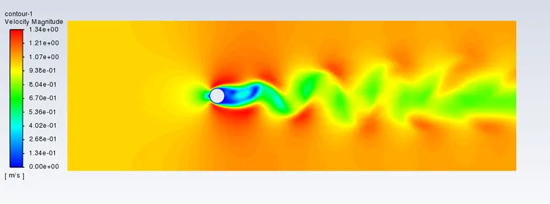
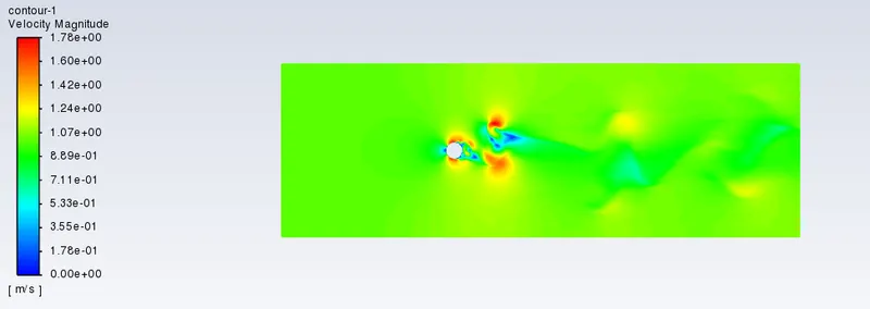
• In the below image we can see vortex shedding behind the cylinder .

Pressure contour :

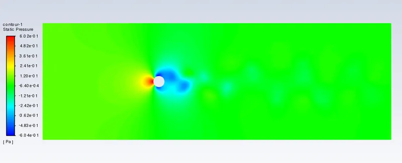
• The below plot is the pressure contour.

• Strouhal number is the frequency at which the velocity oscillates.If we know the time we can calculate the vortex shedding frequency,From which we can calculate the strouhal number. Now we can't calculate the Strouhal Number for steady state because they are used to get the final solution.Any intermediate solution is not time accurate.It means if we get some velocity value at particular iteration it does not relate to particular time .We will not be able to calculate frequency parameter because there is no time parameter.This is the reason we need to run transient simulation ,where we solve equations with respect to time .So at each and every time step we solve the equations accurately and trust the results with respect to time.

Simulating the flow with the transient case :

• From geometry creation to meshing everything is same as steady case for transient case also, the change comes in the problem setup, we use transient solver instead of steady state solver .So let us start from problem setup.

Problem Setup :

• To set up our problem we open Fluent and setup inital conditions , boundary conditions material etc.,
• We first start with checking the mesh quality using perform mesh check under domain.If no error is seen in console window then we can proceed further.
• Then we move move to setting up physics where we select the solver ,viscous model ,initial and boundary conditions etc.,
• We use a steady state pressure based solver to solve our model.

Physics :

General :

Solver type : pressure based

time : transient state

velocity formulation : absolute

• Then we select the viscous model as laminar since the reynolds number is very small the flow will be laminar.

models :

viscous model : laminar

Material :

• Here the way we are going to control our Reynolds number is by modifying the dynamic viscosity of our working fluid.
• The way we do this is in materials we the air and we rename it we change the value of denisty and viscosity of our fluid so that the Reynolds number is equal to 100.

Density = 1 kg/m^3

Viscosity = 0.02 kg/m.s

• Here as our characteristic length is 2 m and we give the inlet velocity value as 1 m/sec we get the Reynolds number =100 .
• This is the condition where we can can surely see the vortex shedding around the cylinder(Karman vortex street).

Zones :

Cell zone : you will see our volume zone which is basically our internal volume basically mesh, and it is of type fluid.We change the material here, which we have just created.

Boundary conditions :We will basically give our boundary conditions here such as inlet velocity and outlet conditions.

we give,

Inlet -x :

velocity : 1 m/sec

Outlet :

pressure outlet : gauge pressure = 0 pa

Cylinder Wall :

wall : No slip

• Now we are almost ready to run the simulation ,but as the solution is being solved we want to moniter different flow quantities while the solution is being generated ,we use definitions for this.
• We want to see vortex average at a point,for that we need a moniter point,we have to create a point.

steps : In results -> create -> point(which we want to create at a distance of 4D from the origin(x = 8 m Y = 0 m from origin)) -> give values -> name it as moniter poin t and click create.

• Now we want to create vortex average at a point .

steps : Definitions -> New -> select the surface report ->vertex average -> field variable : velocity -> velocity magnitude -> under surface -> select the moniter point which we have just created -> check

report file and report plot ->then okay.

• Now we also want to moniter the lift and drag coefficient plot while the solution is being run.

steps : Definitions -> New -> select the force report -> drag -> select cylinder wall under zones -> check report file and report plot -> then okay.

• In the same way create a plot for lift coefficient also.
• we also want to create aminations so that as the solution is changing as the function of time we can see the physics behind it.
• Pressure and velocity contours :
• We want to see the pressure and velocity contour as the solution is being generated. For that we have to initialize the domain first.
• We use the standard initialization from the inlet.Then to create contour we follow below steps ,

For contour -> go to solutions tab -> graphics -> contour -> in contour of : select velocity under that velocity magnitude -> select all the surfaces and press save /display.

• Then you can see the initial values for velocity which is obtained by initialization which is not the final one.
• In the same way create the pressure contour plot also.
• Then we create animation so that we can see how these parameters are varying when problem is being solved.
• In solution method we use coupled .
• In residuals we have continuity , X- velocity ,Y- velocity.We uncheck convergence because we want to see solution till the number of iterations we input ,so that the solving doesn't stop when it gets converged.

Solving :

• Give iterations such that your solution is converged.Not only residuals but also some physical parameters which are important.In our case that could be the velocity in the moniter point location.
• Run the simulation until the steady state is reached.Lets run for 2750 times steps with time step size of 0.1 iterations ,we can find the solution is converged.
• Once it cross 600 time steps you will see the vortex shedding and after 2000 time steps you can observe all the plots has obtained steady state.Then post process the results.
• Then we can see that in the residual plot we see residuals dropping and reach a steady state after 175 iterations.

Post processing :

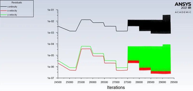
Residuals plot :

• You can observe from the below plot the residuals has converged after 29200 iterations.

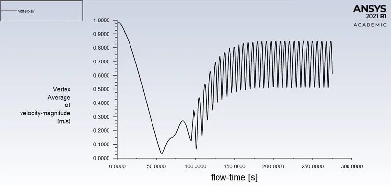
Vortex average plot :

• • You can observe from the below plot that vertex average has reached the steady state as it follows the same pattern after 1750 time steps(175 seconds flow time).So we can conclude that the flow has converged.

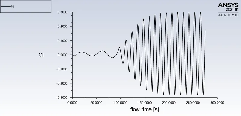
Lift plot :

• You can observe from the below plot that lift coefficient has reached the steady state as it follows the same pattern after 2000 time steps(200 seconds flow time).So we can conclude that the flow has converged.

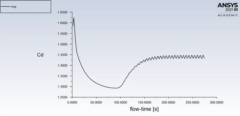
Drag plot :

• You can observe from the below plot that drag coefficient has reached the steady state as it follows the same pattern after 1750 time steps(175 seconds flow time).So we can conclude that flow has converged.

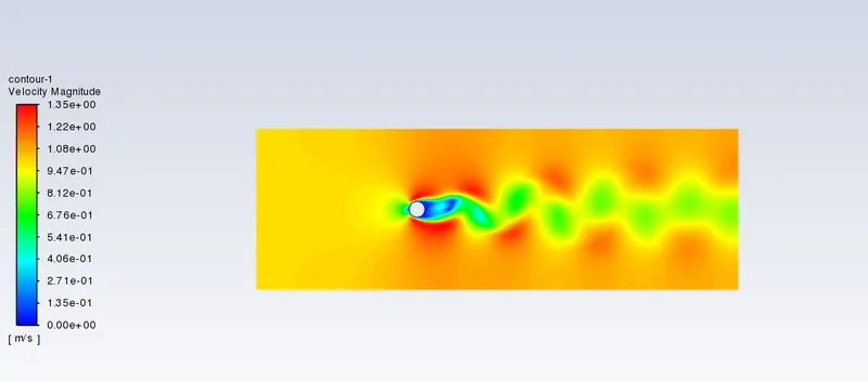
Velocity contour :

• In the below image we can see vortex shedding behind the cylinder .

Pressure contour :

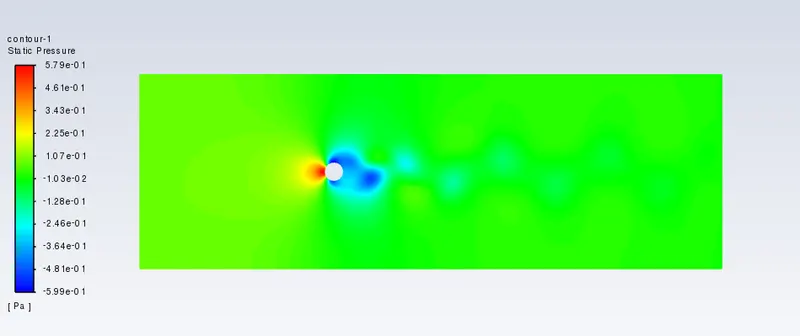
• The below plot is the pressure contour.

Strouhal Number for Re= 100 :

Experimental value :

let us calculate for RE =100

=> st = 0.198(1-(19.7/100))

Therefore, Strouhal number = 0.1589

CFD simulation value :

The Strouhal number is often given as,

where f is the frequency of vortex shedding,

L is the characteristic length and

U is the flow velocity.

From the lift plot you can calculate frequency of vortex shedding, f =no of full cycles/time period = 4/50 = 0.08

L is the characteristic length = 2 m

U is the flow velocity = 1m/sec

Strouhal number = 0.08 *2/1 = 0.16

• Therefore our CFD result Strouhal number is almost equal to the experimental value.

Calculation of coefficient of drag and lift over a cylinder for the Reynolds number to 10,100,1000,10000 & 100000 :

• Let us simulate the above case with steady state solver for different Reynolds number to find out how coefficient of drag and lift varies over a cylinder.

• Case -1) RE = 10 :

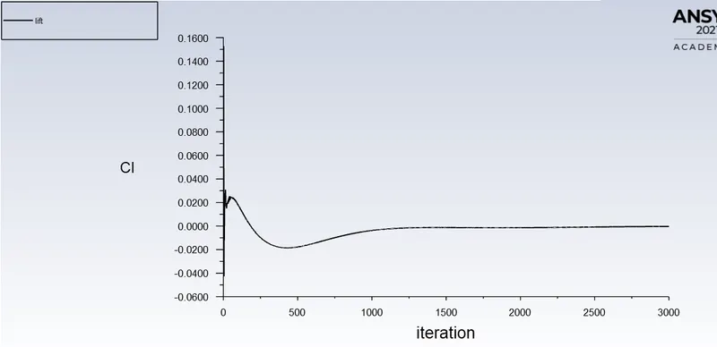
  Lift plot :

• You can observe from the below plot the lift coefficient has converged and reached a steady state and value of lift coefficient is -0.0003.

• 

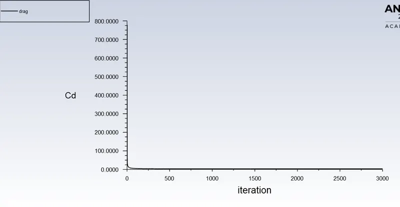
  Drag plot :

• You can observe from the below plot the drag coefficient has converged and reached a steady state and value of drag coefficient is 3.33.

• 

  Velocity contour :

• In the below velocity plot we can see vortex shedding behind the cylinder .

• 

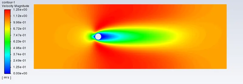
Case -2) RE = 100 :

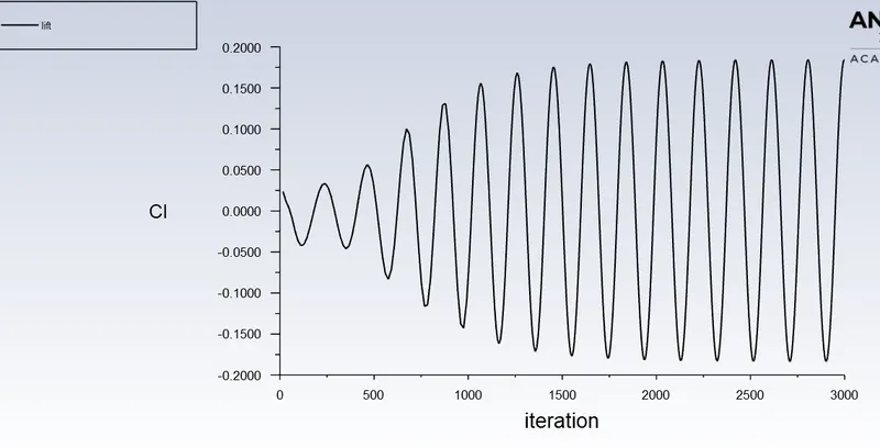
Lift plot :

• You can observe from the below plot the lift coefficient has converged and reached a steady state and value of lift coefficient is 0.184.

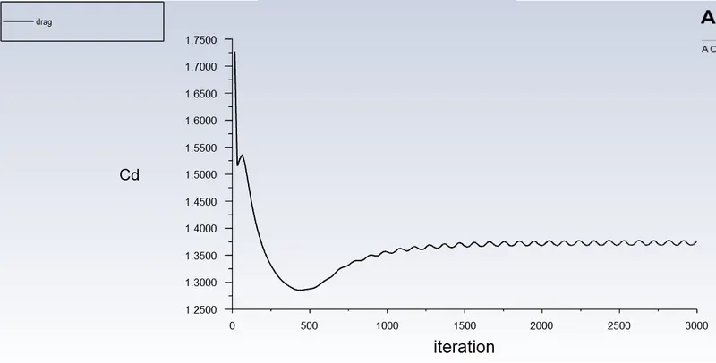
Drag plot :

• You can observe from the below plot the drag coefficient has converged and reached a steady state and value of drag coefficient is 1.37.

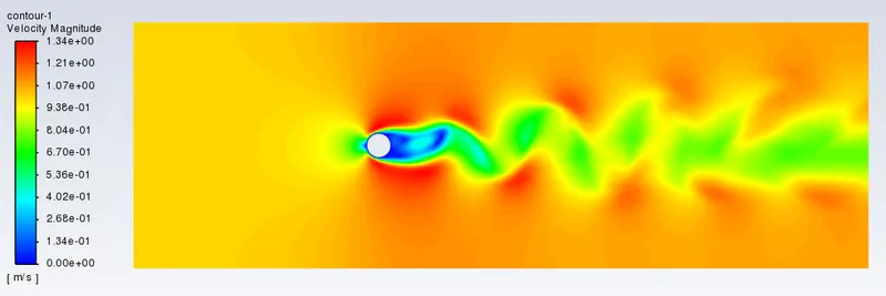
Velocity contour :

• In the belowvelocity plot we can see vortex shedding behind the cylinder .

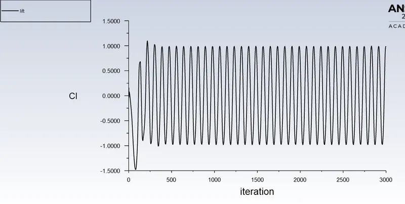
Case -3) RE = 1000 :

Lift plot :

• You can observe from the below plot the lift coefficient has converged and reached a steady state and value of lift coefficient is 0.98.

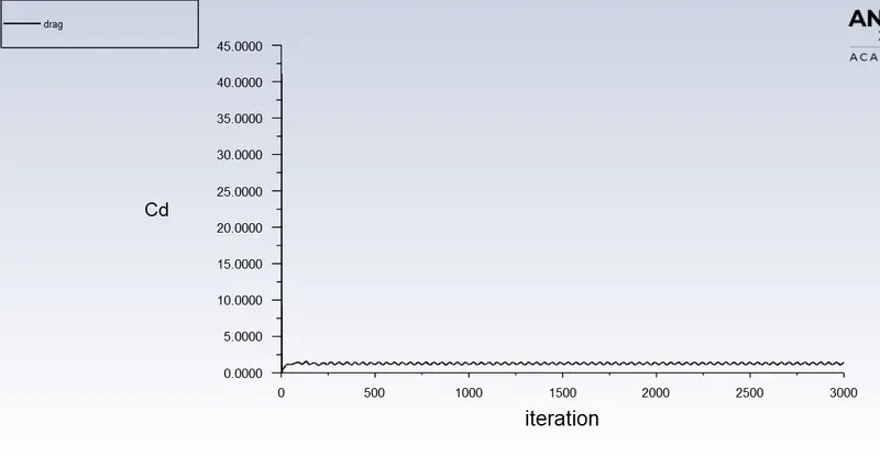
Drag plot :

• You can observe from the below plot the drag coefficient has converged and reached a steady state and value of drag coefficient is 1.31.

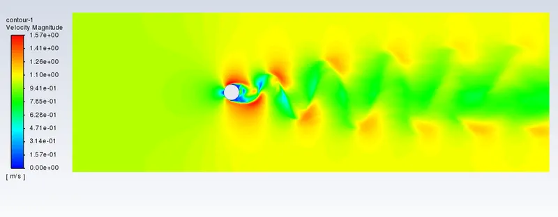
Velocity contour :

• In the belowvelocity plot we can see vortex shedding behind the cylinder .

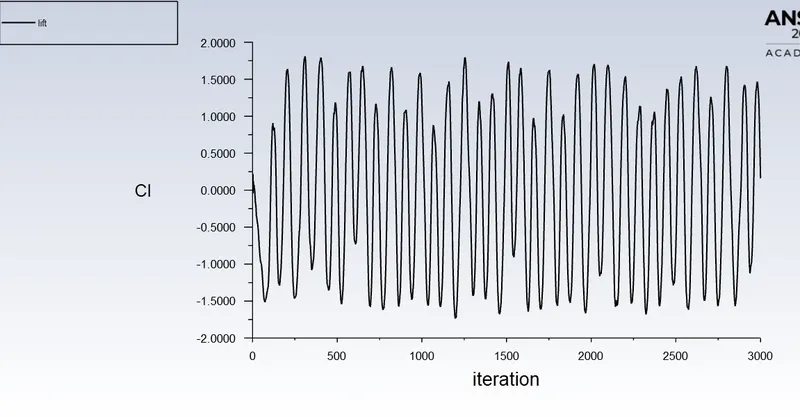
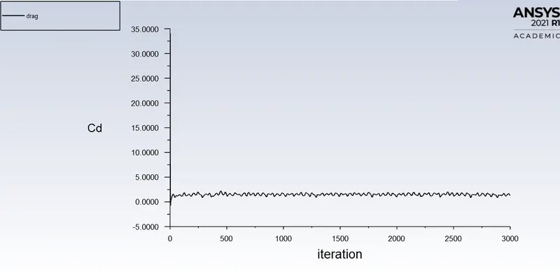
Case -4) RE = 10000 :

Lift plot :

• You can observe from the below plot the lift coefficient has converged and reached a steady state and value of lift coefficient is 1.3.

Drag plot :

• You can observe from the below plot the drag coefficient has converged and reached a steady state and value of drag coefficient is 1.21.

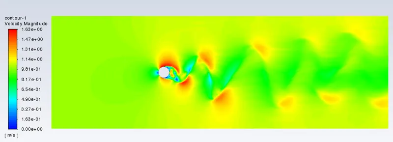
Velocity contour :

• In the below velocity plot we can see vortex shedding behind the cylinder .

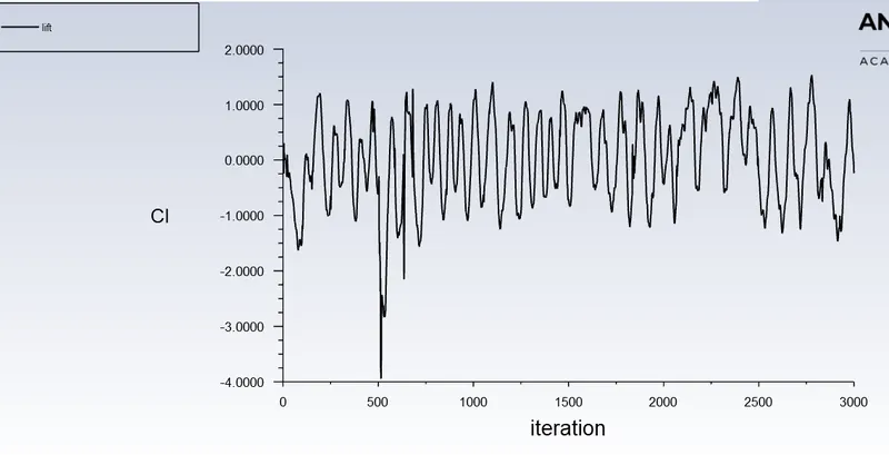
Case -5) RE = 100000 :

Lift plot :

• You can observe from the below plot the lift coefficient has converged and reached a steady state and value of lift coefficient is 0.99.

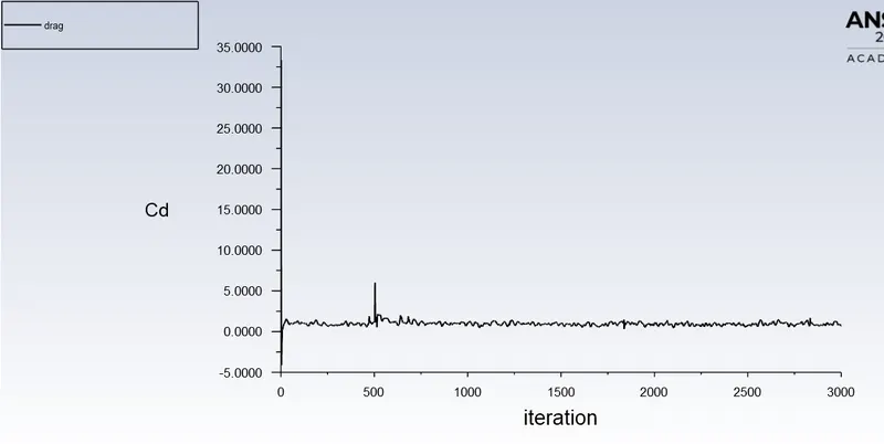
Drag plot :

• You can observe from the below plot the drag coefficient has converged and reached a steady state and value of drag coefficient is 0.98.

Velocity contour :

• In the belowvelocity plot we can see vortex shedding behind the cylinder .

Effect of Reynolds number on the coefficient of drag :

• Let us tabulate all the values and discuss the effect of Reynolds number on the coefficient of drag.

• The drag coefficient decreases at low Reynolds numbers because the flow is in a regime called creeping flow. That is, the inertial forces are negligible.Drag is a sum of friction drag and pressure drag.At very low reynolds number the flow is full attached ,the drag is due to skin friction drag and as reynolds number increases there will be increase in pressure drag due to seperation.When flow turns to turbulent again there the flow will be more attached this causes decrease in pressure drag but eventually leads to increase in friction drag.Lets discuss this more briefly.
• At RE =10 illustrates what actually occurs for low velocity. A stable pair of vortices are formed on the downwind side of the cylinder. The flow is separated but steady and the vortices generate a high drag on the cylinder or sphere.
• AT RE = 100 shows the flow as velocity is increased. The downstream vortices become unstable, separate from the body and are alternately shed downstream. The wake is very wide and generates a large amount of drag. The alternate shedding is called the Karman vortex street.This type of flow is periodic, it is unsteady but repeats itself at some time interval. The pressure variation associated with the velocity changes produces a sound called an aeolian tone. This is the sound you hear when the wind blows over high-power wires or past tree limbs in the fall or winter. It is a low frequency (low pitch), haunting tone.
• AT RE = 1000 and 10000 shows the flow as the velocity is increased even more. The periodic flow breaks down into a chaotic wake. The flow in the boundary layer on the windward side of the cylinder is laminar and orderly and the chaotic wake is initiated as the flow turns onto the leeward side of the cylinder. The wake is not quite as wide as for RE =100, so the drag is slightly less.
• The large dive in the drag coefficient is called the drag crisis. This happens when the boundary layer over the cylinder transitions from laminar to turbulent. Turbulent boundary layers are more resistant to separation, so the flow stays attached longer resulting in decreased form drag.
• In between RE = 100000 and 1000000 shows the flow at even higher velocity. The boundary layer transitions to chaotic turbulent flow with vortices of many different scales being shed in a turbulent wake from the body. The separation point is initially slightly downstream from the laminar separation point, so the wake is initially slightly smaller and the drag is less than the corresponding laminar drag. there is a range of Reynolds numbers, during transition from laminar to full turbulent, for which the turbulent drag is less than the laminar drag i.e., after RE = 10^5 there is large dive in the drag coefficient is called the drag crisis. This happens when the boundary layer over the cylinder transitions from laminar to turbulent. Turbulent boundary layers are more resistant to separation,so the flow stays attached longer resulting in decreased form pressure drag.
• Increasing velocity eventually brings the turbulent drag up to and even higher than the laminar drag value i.e., after 10^6 Reynolds number the drag coefficient rises again as more and more of the cylinder has a turbulent boundary layer. Turbulent boundary layers have a higher skin friction coefficient than their laminar counterparts.
• All of the calculations shown for the cylinder have employed a smooth surface. But since drag depends on the flow in the boundary layer, we can expect some changes with surface roughness. It is observed experimentally that a roughened cylinder or ball will transition to turbulent flow at a lower Reynolds number than a smooth cylinder or ball.This effect produces a rather interesting result. There is a small range of Reynolds numbers for which the drag of a roughened ball is less than the drag of a smooth ball for the same diameter,velocity and flow conditions.The size and speed of a golf ball falls within this Reynolds number range.That is why a golf ball has dimples; the roughened surface causes transition to turbulence that would not occur yet on a smooth golf ball. The lower drag on the dimpled golf ball allows the ball to fly farther than a smooth ball of the same speed,diameter and weight.

Animation of vortex shedding :