Week 6 - CHT Analysis on a Graphics card

In this challenge,

• We will ,give a brief description of why and where a CHT analysis is used.

• We will Perform a steady-state conjugate heat transfer analysis on a model of a graphics card by using appropriate materials for the simulation.

• We then vary the velocity from 1 m/sec to 3 m/sec and 5 m/sec for 3 velocities and discuss the results.

• We find out the maximum temperature and heat transfer coefficient attained by the processor.

• We then finally prove that the simulation has achieved convergence with appropriate images and plots and Identify potential hotspots on the model.

Conjugate Heat Transfer (CHT) analysis :

Conjugate Heat Transfer analysis allows for the simulation of heat transfer between solid and fluid domains by exchanging thermal energy at the interfaces between them and transported via conduction within solids and adiditionally via convection within fluid domains.Conjugate heat transfer analysis can accurately predict heat transfer by simultaneous solving all the relevant solid and flow field heat transfer processes.Conjugate heat transfer corresponds with the combination of heat transfer in solids and heat transfer in fluids. In solids, conduction often dominates whereas in fluids, convection usually dominates. Conjugate heat transfer is observed in many situationsfor example: conduction through solids, free and forced convection in the gases/fluids and thermal radiation.

• The three main modes of heat transfer:
  ‐ Conduction is heat transfer that occurs when a temperature difference exists across a stationary medium.
  ‐ Convection is the heat transfer between a surface and a moving fluid when there is a temperature difference between the two.
  ‐ Radiation(thermal radiation) is the emission of energy in the form of electromagnetic waves. In the absence of an intervening medium ,there is net heat transfer by radiation between two surfaces at different temperatures.

Conduction :

• Conduction is thermal energy transmission through solid or fluid by the action of translational, rotational and vibrational motion of atoms and molecules.
• Molecular collisions transfer energy from more energetic molecules to less energetic ones. Higher temperature = Increased atomic/molecular motion
• Conduction occurs in all fluid and solid media.
• Due to the Second Law of thermodynamics, heat must always be conducted from higher to lower temperatures.
• Conduction problems often involve fluid flows at the boundaries of the solid, which serve as a mechanism for heating or cooling the solid.
• Conduction is the transfer of energy from more energetic to the less energetic particles of a substance via interactions between the particles at molecular levels due to a temperature difference.
• Temperature at any point can be associated with the energy of random translational, internal rotational and vibrational motions of gas molecules.
• Molecular collisions transfer energy from more energetic molecules to less energetic ones .
• Higher molecular energies are associated with higher temperatures, and the energy transfer always occurs in the direction of decreasing temperature in the presence of a temperature gradient.
• The mechanism of conduction is the same for liquids as the molecules are closely spaced and the molecular interactions are stronger and more frequent than gases.
• In the case of solids, conduction is associated with atomic activity in the form of lattice vibrations. In the case of an electrical conductor, the translational motion of free electrons also contributes to energy transfer.
• The heat transfer process can be quantified in terms of appropriate rate equations which are used to compute the amount of energy being transferred per unit time.
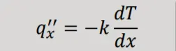
• In the case of heat conduction, the rate equation is Fourier’s law. For a one-dimensional plane wall
  this is expressed as

• Here,
  ‐ 𝑞_𝑥^′′(𝑊/𝑚^2) is the heat transfer rate per unit area in the x-direction.
  ‐ 𝑘 is the thermal conductivity (𝑊/𝑚𝐾) and is a characteristic of the wall material.
  ‐ The negative sign signifies the fact that the heat transfer is in the opposite direction of the temperature gradient

Convection :

• Convection is transfer of heat by the combination of the bulk motion of a fluid and random molecular motion (diffusion).
• Heat is transferred to/from the fluid via conduction at walls.
• Fluid carries thermal energy to other parts of the system.
• Heat transfer only due to the bulk motion of the fluid (no diffusion) is referred to as advection.
• Convection heat transfer can be classified into:
• Forced convection: Flow is caused by external means, such as by a fan, a pump or atmospheric winds.
• Free (or natural) convection: Flow is induced by buoyancy forces, caused by density differences due to the temperature variations in the fluid.
• Mixed (combined) connection: Forced and natural convection can also exist if both external driving forces and buoyancy forces exist.
• Heat transfer by convection is rooted in the idea that the heat transfer rate is proportional to the temperature difference between a fluid and a heated/cooled body.
• This idea is called Newton’s Law of Cooling. The parameter governing the rate of heat transfer is the heat transfer coefficient, usually denoted ℎ.

Here, 𝑞′′ = Convective heat flux
𝑇𝑠= Temperature of the solid surface
𝑇∞= Temperature of the fluid

• One of the central problems in convection is determining the heat transfer coefficient for a given flow field.
• The heat transfer coefficient depends on the conditions in the boundary layer, and it is affected by the surface geometry, the nature of the fluid flow and various fluid thermodynamic and transport properties.

Radiation Heat Transfer :

• Thermal radiation heat transfer is the emission of energy via electromagnetic waves.
• All matter at a nonzero temperature emits thermal radiation.
• This emission is due to changes in the electron configurations of the atoms or molecules, and the energy is transported via electromagnetic waves (or photons).
• Radiation intensity depends on body temperature and surface characteristics.
• Unlike conduction or convection, radiation does not require the presence of a material medium and can occur in a vacuum.
• Radiation is an important mode of heat transfer at high temperatures.
• It is also the only mode of heat transfer in outer space, and this is how the solar energy reaches Earth.

Heat transfer in solids and heat transfer in fluids are combined in the majority of applications. This is because fluids flow around solids or between solid walls, and because solids are usually immersed in a fluid. An accurate description of heat transfer modes, material properties, flow regimes, and geometrical configurations enables the analysis of temperature fields and heat transfer. Such a description is also the starting point for a numerical simulation that can be used to predict conjugate heat transfer effects or to test different configurations in order, for example, to improve thermal performances of a given application.

Introduction :

• Here we will Perform a steady-state conjugate heat transfer analysis on a model of a graphics card by using aluminum for the all other materials other than processor because aluminum is used to create an effective fin formation medium for transferring heat in many industrial and haet transfer applications. Aluminum is chosen because of its inherent light weight, increased conductivity, and easy malleability. It is also a superior choice when the application involves exposure to environmental conditions, liquids, and/or chemicals because of its inherent resistance to corrosion.Because of these properties, industries such as aerospace, automotive, and HVAC choose aluminum fin stock as their preferred material for radiators, evaporators, coolers, heaters, and condensers.
• And for processor we use the silicon, because, silicon is used for electronic devices because it is an element with very special properties. One of it’s most important properties is that it is a semiconductor. This means that it conducts electricity under some conditions and acts as an insulator under others. Silicon’s electrical properties can be modified through a process called doping. These characteristics make it an ideal material for making transistors that amplify electrical signals.Silicon’s properties are not the only reason why it is ideal for electronic devices. Silicon is also an abundant element on Earth. It is even the most common element in the Earth’s crust. The abundance of Si allows it to be extremely affordable and appealing. It is no wonder why silicon has become the basis of memory chips, computer processors, transistors, and all other electronics.
• As electricity passes through the CPU or gets blocked inside, it gets turned into heat energy. While a processor in a high-performance workstation may run hot due to heavy use, a processor in a regular computer that overheats is almost always a sign of a malfunctioning system.So its mandatory for cooling the processor.
• The heat from processor is transferred to fins by conduction,as fins are attached to it and then by forced convection we remove heat by using air as a coolant from the processor and fins to cool the heated processor.

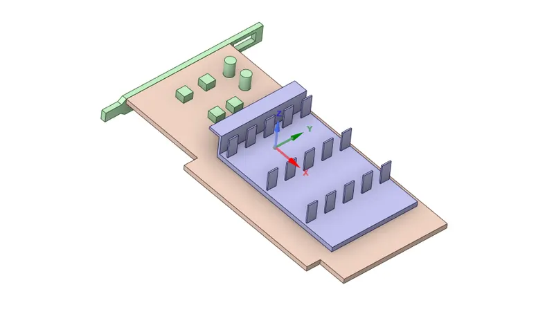
• Here we need to calculate required parameters for three cases i.e., for threevelocities 1 m/sec, 3 m/sec and 5 m/sec .Let us solve for one by one.

Case -1 : 1m/sec :-

Solution procedure :

• We wil simulate both fluid flow and also the heat transfer to the solid i.e., CHT Analysis on an Exhaust port with the steady state .Then for solving we follow the below procedure :

1)Geometry setup

2)Meshing

3) Problem setup

4)Solving

5)Post processing

• Then we calculate the wall/surface heat transfer coefficient on the internal solid surface & show the velocity & temperature contours in appropriate areas.

Simulating the flow with the Steady case :

In the ANSYS work bench we first open the fluent module by drag and drop.The we follow the procedure we have mentioned above

1) Geometry setup :

• In fluent module we have to open spaceClaim and import the geometry.If you hide the enclosure you can see the graphics card.

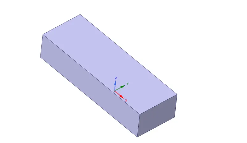
• If you mesh it now it will be non conformal,So as mesh needs to be conformal i.e., the edges need to be connected exactly then only the heat is going to transfer smoothly.We need to share topology for that, then only the mesh will be uniform and with perfect connectivity.
• Now enable the share toplology and then go to work bench and select all the components including enclosure and then click share .This is very important if you don't do this step you will not see the single interface between them.So this particular step takes care of creating the interfaces,so that you will have one interface between all the parts of the geometry.Once you have done this you will see the pink and blue lines at the interface,that basically tells you where the things are being shared.Basically what this means is that you will have a sharing between inner wall of solid and outer layer of fluid will have a common interface and bounds of share is one.This is only interface you will see.

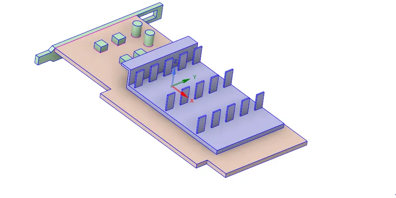
• Now if you open meshing and you will see that there is perfect mesh connectivity and the interface is shared perfectly.This is exactly how we need to make meshes for CHT simulation.
• This completes the creation of geometry.Then we close the spaceClaim ,the progress will be saved automatically.

2) Meshing :

• For meshing we open Meshing,where we mesh our model so that we can use it to solve our model.
• In general it is always good to name the surfaces before meshing. So let us do that.
• We first select the entity by using the entity selection so that we can provide name for our entity selection.

steps : select the body you want to name by using body selection -> then press N -> name the selection.

• In the similar way we name fins,capacitors,base,processor and inlets,outlet(by face selection)
• Then next thing to do is to mesh.We click the mesh option in the side window and create our base line mesh.We then refine mesh.Let's mesh the geometry .Once the mesh has done we need to see what are the things we have to refine.Let us refine one by one.

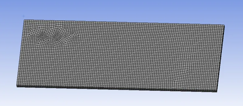
a) Method (Multizone method) :

• Now comming to the refining mesh if you see the main base which the fins and processor are there there is a perfect structure made of straight lines i.e., no complex shape ,in 3D made of boxes.So when you have such a scenario like this it is better to use hexahederal mesh.Hexahederal meshes have the highest quality of all the mesh types so whenever it is possible it is better to use that.
• So to do this ,we right click mesh => insert =>insert => method =>in geometry - select base => Apply for method - multizone(Whenever you use multizone it creates hexa meshes wherever it is possible and in another regions where it is having different mesh type it is going to have perfect connectivity)

b)Main body sizing(Body sizing) :

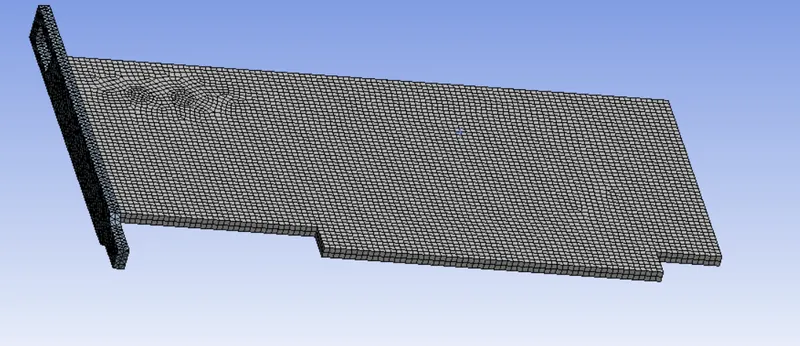
• As to capture the exact distribution of heat by the conduction and also to calculate the temperature exactly we need to make the mesh of body finer by using sizing.To do this,
• Right click on mesh => sizing => in geometry -we select the base and give size of 0.5 mm => Then generate mesh again you will the mesh is finer.

c) Processor sizing(Body sizing) :

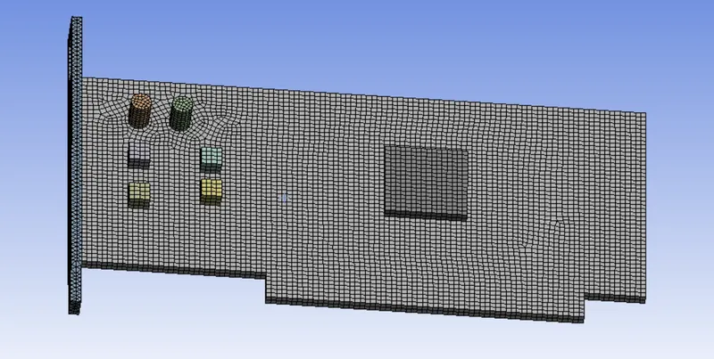
• As for exact distribution of heat source we need to make the mesh of processor finer by using sizing. To do this,
• Right click on mesh => sizing => in geometry -we select processor and give size of 0.5 mm => Then generate mesh again you will seethe processor is refined finer.

d) Capacitor sizing(Body sizing) :

• We are making the mesh of capacitor finer as they should get exact shape and also the heat transfer to them should also be calculated exactly to refine them we using sizing.To do this,
• Right click on mesh => sizing => in geometry -we select all capacitors and give size of 0.5 mm. and also select yes for curvature capture. => Then generate mesh again you will see the shape of capacitors is exactly captured and also refined finer.

e) Fins sizing(Body sizing) :

• As to capture the exact distribution of heat by the conduction to fins and convection through and also to calculate the temperature exactly we need to make the mesh of fins finer by using sizing.To do this,
• Right click on mesh => sizing => in geometry -we select the base and give size of 0.6 mm => Then generate mesh again you will the mesh is finer.

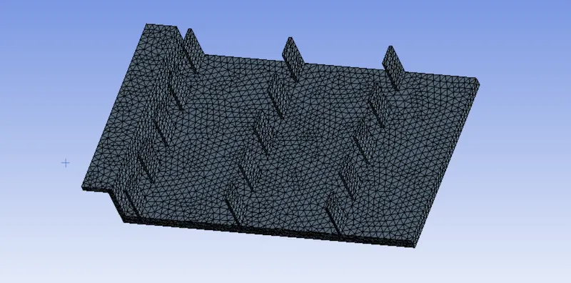
• Below is the view of the final mesh.

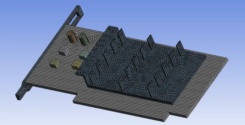
f) Enclosure sizing :

• Now we have to refine the enclosure for that give a size of 6mm in global mesh size then you will see the enclosure is also refined.

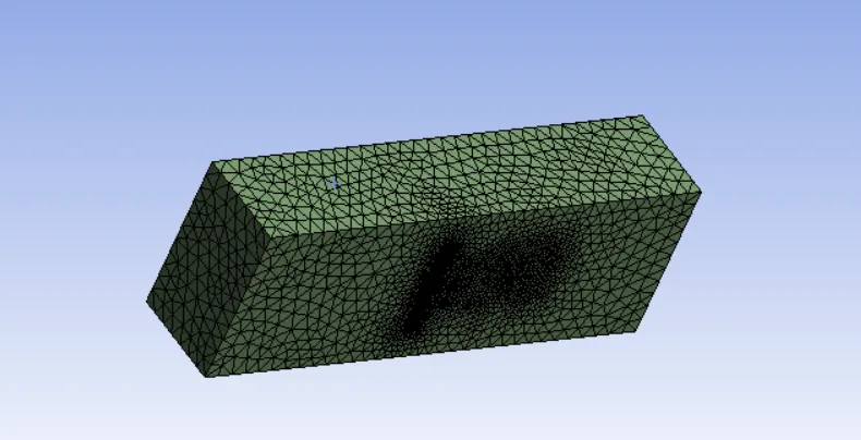
• Now we have to check the quality of the mesh.steps : mesh ->quality-> mesh metric-> Element quality
• Here our minimum quality is around 18 %,so we can move further for our solution setup.

3) Problem Setup :

• To set up our problem we open Fluent and setup inital conditions , boundary conditions material etc.,
• We first start with checking the mesh quality using perform mesh check under domain.If no error is seen in console window then we can proceed further.
• Then we move move to setting up physics where we select the solver ,viscous model ,initial and boundary conditions etc.,
• We use a steady state pressure based solver to solve our model.

Physics :

General :

Solver type : pressure based

time : steady state

velocity formulation : absolute

models :

viscous model : k-omega SST

Material : Fluid : Air

Solid : aluminum(for all components except processor) ,silicon (for processor-we select any other element and change the name to silicon and give properties of silicon)

• As temperature is also required we need to select energy equation.

Zones :

Cell zone :

• In cell zones you will see fluid volume it is of type fluid with material air ,and in solid volume we can see the named selection we have gave in meshing,and we give aluminum as material for all components except processor ,and silicon as material for processor.
• Here for processor we give internal heat generation as source term, we will not give it boundary condition because if you give there it will be constant around whole domain and when you give it in cell zone it will be given or generated at the centre and spread around whole processor.
• As we know that, Heat flux (Ф) can be defined as the rate of heat energy transfer through a given surface (W)which is 60W from the processor , and heat flux density (φ) is the heat flux per unit volume (W/m3),which we give as input for internal heat genration i.e, 60/6.4e-08( as we know the volume of processor = 6.4e-08 m^3).So the internal heat generation is given as 937500000 W/m^3.

Boundary conditions :We will basically give our boundary conditions here such as inlet velocity and outlet conditions.

we give,

Inlet :

velocity : 1 m/sec

temperature : 293 K(room temperature)

Outlet :

pressure outlet : gauge pressure = 0 pa

• Now if you check other BC they are just wall boundaries ,To couple the two sides of the wall, they need to be set to coupled option under Thermal Conditions.But,here we are not changing anything they are already set to coupled condition for thermal BC.
• Now we are almost ready to run the simulation ,but as the solution is being solved we want to moniter different flow quantities while the solution is being generated ,we create contour for this.But before that we have to initialize the domain.We use the Standard initialization from inlet, this provides a very good initial condition .
• Now we want to see the temperature contour.
• For contour -> go to solutions tab -> graphics -> contour -> in contour of : select temperature under that select static temperature -> select all the walls (all parts of graphics card)and press save /display.
• Then you can see the initial values for temperature for whole domain which is obtained by initialization which is not the final one.
• Then we want to create animation so that we can see how the temperature is varying over the domain when problem is being solved.
• For that,

steps : Activities -> solution animation -> select temperature contour,which we have created -> preview -> set the required view and use active -> and name it as temperature animation.

• In solution method we use SIMPLE .

4) Solving :

• Give iterations such that your solution is converged.
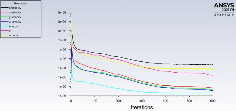
• Run the simulation until the steady state is reached.Lets run for 600 iterations ,we can find the solution is converged.
• Then we can see that in the residual plot that residuals dropping and reach a steady state after 550 iterations.
• Then let us post process the results.

5)Post processing :

Residuals plot :

• You can observe from the below plot the residuals has converged after 550 iterations.

Temperature contour :

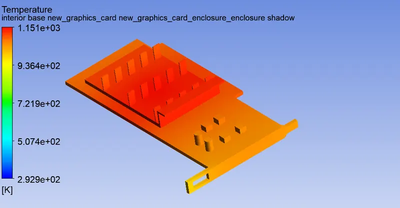
• The below plot is the temperature contour on graphics card.You can see that there are very high temperature regions near to the processor this is mainly due to the conduction.

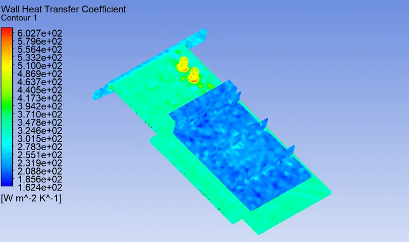
Heat transfer coefficient contour :

• The below plot is the heat transfer coefficient contour contour on graphics card.Here you can observe that the maximum heat transfer due to convection is to the cylinderical shape capacitors and this is mainly due to their shape , as we know heat transfer coefficient depends on area.And this value incrases as velocity increases.

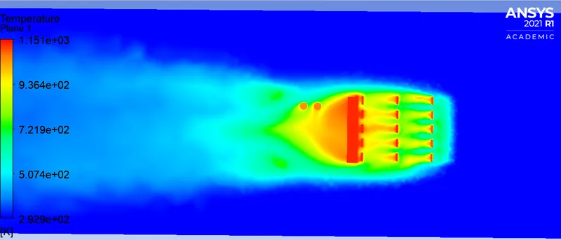
Mid-plane temperature contour :

• The below plot is the temperature contour on graphics card on a midplane.You ca bserve that that the temperature is high at the end of fins this is mainly due to recirculation region.You can observe this more clearly in the velocity contour.

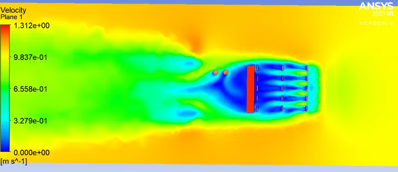
Mid-plane velocity contour :

• The below plot is the velocity contour of flow over graphics card plotted on a midplane.Where the graphics plate has temperature plotted on it.You can see that the velocity of air at the end of fins is almost zero ,this is due to recirculation region .We can clearly observe this when we plot the vectors.

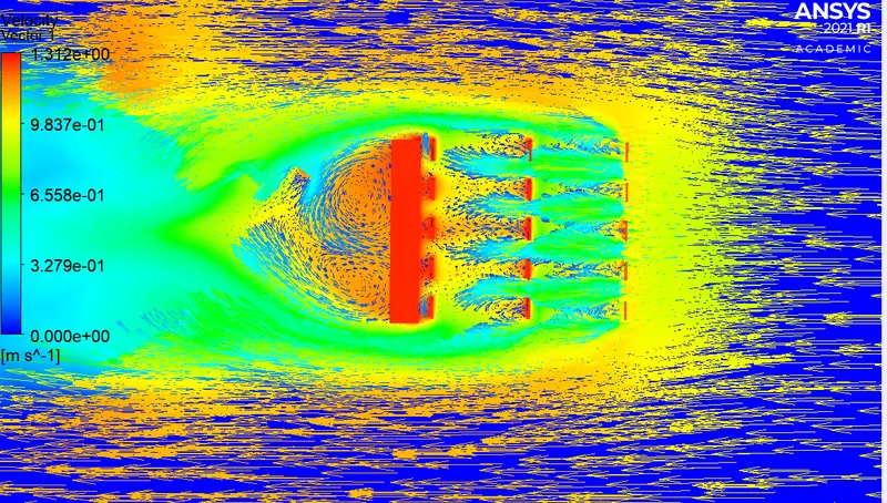
Velocity vector contour on mid-plane :

• The below plot is the velocity vectors plotted on a midplane where temperature is plotted on midplane and graphics card.You can see that the high temperature region is at the end of fins .You can observe it clearly at the location where there is a recirculation zone,where velocity of air is almost zero.

Case -2 : 3 m/sec :-

• In this case everything is same from the point of geometry and also in meshing everything is same as above case.
• Comming to set up the change comes here.
• Here when it comes to setup we give inlet velocity as 3 m/sec and remaining everything is same.
• So let us directly run the simulation then postprocess the results and compare in between the results.

Residuals plot :

• You can observe from the below plot the residuals has converged after 450 iterations.

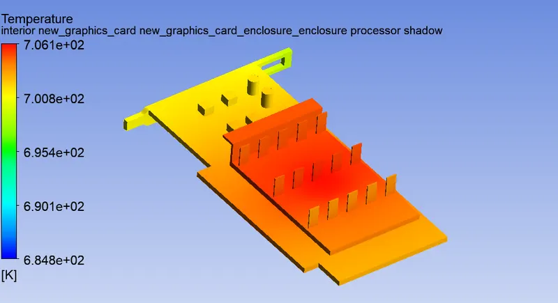
Temperature contour :

• The below plot is the temperature contour on graphics card.You can see that there are very high temperature regions near to the processor this is mainly due to the conduction.

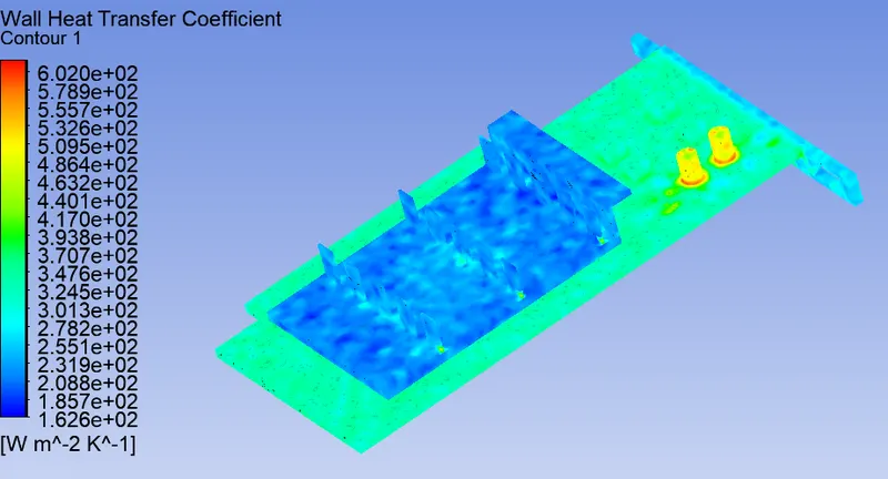
Heat transfer coefficient contour :

• The below plot is the heat transfer coefficient contour contour on graphics card.Here you can observe that the maximum heat transfer due to convection is to the cylinderical shape capacitors and this is mainly due to their shape , as we know heat transfer coefficient depends on area.And this value incrases as velocity increases.

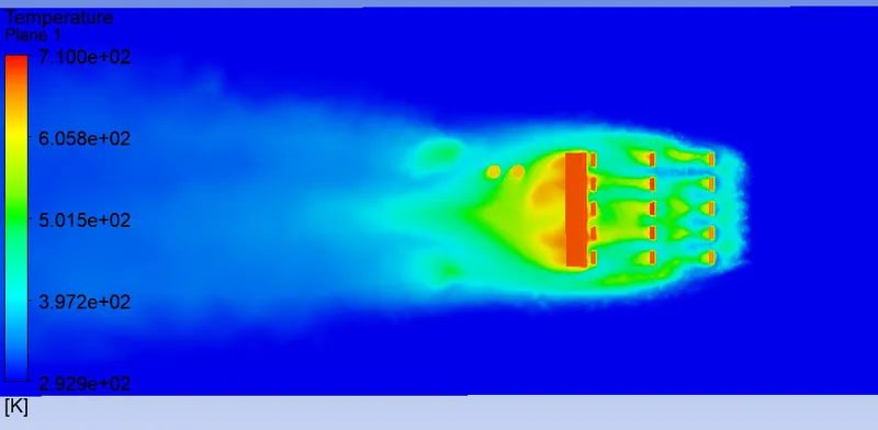
Mid-plane temperature contour :

• The below plot is the temperature contour on graphics card on a midplane.You ca bserve that that the temperature is high at the end of fins this is mainly due to recirculation region.You can observe this more clearly in the velocity contour.

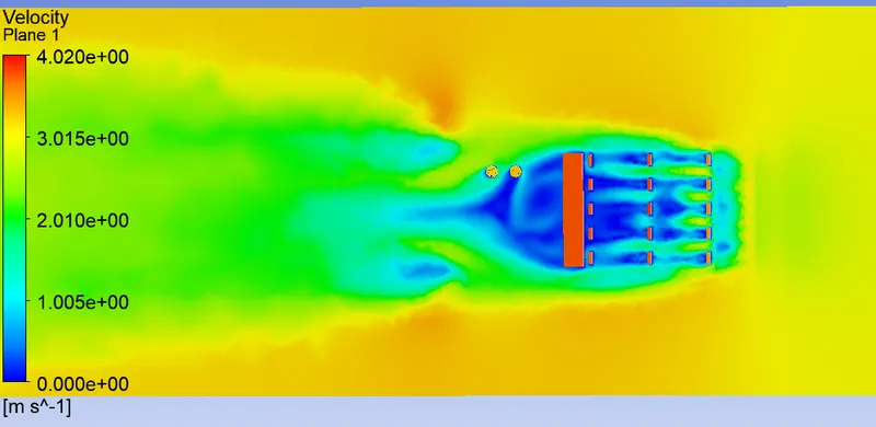
Mid-plane velocity contour :

• The below plot is the velocity contour of flow over graphics card plotted on a midplane.Where the graphics plate has temperature plotted on it.You can see that the velocity of air at the end of fins is almost zero ,this is due to recirculation region .We can clearly observe this when we plot the vectors.

Case -3 : 5 m/sec :-

• In this case everything is same from the point of geometry and also in meshing everything is same as above two cases.
• Comming to set up the change comes here.
• Here when it comes to setup we give inlet velocity as 5 m/sec and remaining everything is same.
• So let us directly run the simulation then postprocess the results and compare in between the results.

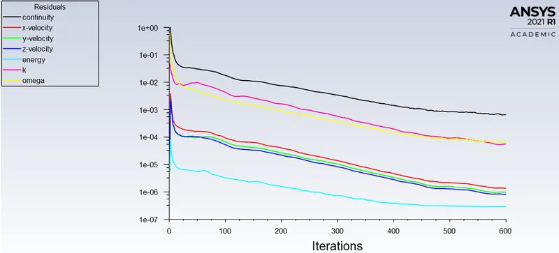
Residuals plot :

• You can observe from the below plot the residuals has converged after 575 iterations.

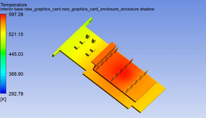
Temperature contour :

• The below plot is the temperature contour on graphics card.You can see that there are very high temperature regions near to the processor this is mainly due to the conduction.

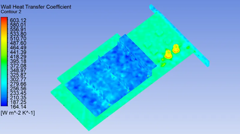
Heat transfer coefficient contour :

• The below plot is the heat transfer coefficient contour contour on graphics card.Here you can observe that the maximum heat transfer due to convection is to the cylinderical shape capacitors and this is mainly due to their shape , as we know heat transfer coefficient depends on area.And this value incrases as velocity increases.

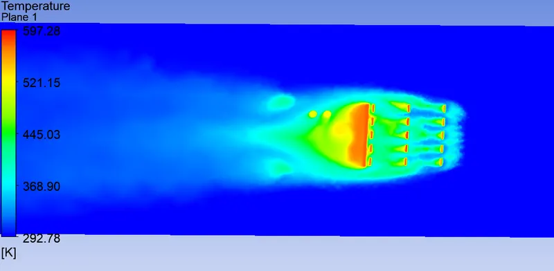
Mid-plane temperature contour :

• The below plot is the temperature contour on graphics card on a midplane.You ca bserve that that the temperature is high at the end of fins this is mainly due to recirculation region.You can observe this more clearly in the velocity contour.

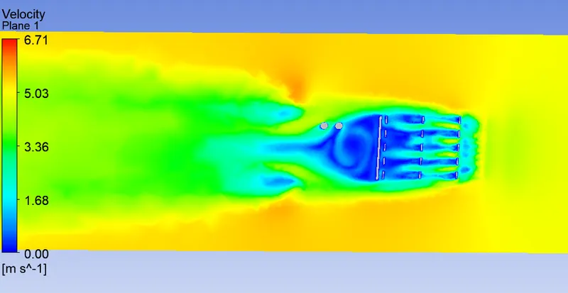
Mid-plane velocity contour :

• The below plot is the velocity contour of flow over graphics card plotted on a midplane. You can see that the velocity of air at the end of fins is almost zero ,this is due to recirculation region .We can clearly observe this when we plot the vectors.

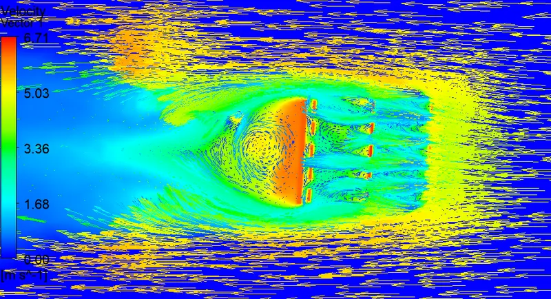
Velocity vector contour on mid-plane :

• The below plot is the velocity vectors plotted on a midplane where temperature is plotted on midplane and graphics card.You can see that the high temperature region is at the end of fins .You can observe it clearly at the location where there is a recirculation zone,where velocity of air is almost zero.

Verifying the HTC predictions from the simulations :

• Let us list out the maximum temperature and heat transfer coefficient attained by the processor in all the cases,

• The Nusselt number is the ratio of convective to conductive heat transfer across a boundary.

• where h is the convective heat transfer coefficient of the flow, L is the characteristic length, k is the thermal conductivity of the fluid.
• Then this Nusselt number is related to Reynolds number i.e.,

• Where ,

and u is the flow speed (m/s)

• So if you observe heat transfer coefficient is directly proportional to the Reynolds number (also to the velocity). So if you increase the velocity then there will be increase in the convective heat transfer coefficient. That's what we can see that the results we got above and if you want you can run another simulation by increasing the velocity of the flow then you will observe there will be increase in the convective heat transfer coefficient of the processor or at a particular location than in the previous low velocity simulation.Hence we can conclude that the results we obtained in the simulation are accurate.

Potential hotspots on the model :

• By seeing the plots of HTC and temperature we can conclude that the potential hotspots on the model are at the cylinderical shape capacitors.The maximum heat transfer due to convection is to the cylinderical shape capacitors and this is mainly due to their shape , as we know heat transfer coefficient depends on area.And this value incrases as velocity increases.You can also observe that there are very high temperature regions near to the processor this is mainly due to the conduction.And if you see the that there is high temperature in the recirculation zone and if you keep any component in that zone it may lead to failure of the component.

Factors that the accuracy of the prediction depend on :

• The factors that the accuracy of the prediction depend on are
• We need to make sure that share topology is set to share.Only then the meshing is going to be uniform and with perfect connectivity.
• We need to select exact turbulent model.As it is wall bounded flow k- omega SST will be very much suitable.And when selecting the turbulence model selecting exact Y+ value also important.
• We need to enable share(share prep) in the work bench for all the components and click share .This is very important if you dont do this step you will not see the single interface between them.So this particular step takes care of creating the interfaces,so that you will have one interface between your solid volume or block and fluid block.

Animations :

• Variation of temperature on Graphics card animation(Steady state) -1 :

• Variation of temperature on Graphics card animation(Steady state) -2 :