Simulating a 2nd order ODE system of a simple pendulum

Objective : Our objective here is to write a program that solves the following ODE. This ODE represents the equation of motion of a simple pendulum with damping.

Theory :A simple pendulum consists of a mass m hanging from a string of length l and fixed at a pivot point and damping coefficient b,when displaced to an initial angle and released, the pendulum will swing back and forth with periodic motion. By applying Newton's secont law for rotational systems, the equation of motion for the pendulum with damping may be obtained by,

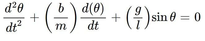
then, drag force of air causes the damping of the simple pendulum. The air exerts a drag force (or resistance) on the pendulum due to which some energy is continuously lost and thus the pendulum comes to rest finally.

In the above equation,

g = gravity in m/s^2,

l = length of the pendulum in m,

m = mass of the ball in kg,

b=damping coefficient.

where we use,

L=1 metre,m=1 kg,b=0.05,g=9.81 m/s2.

and we simulate the motion between 0-20 sec, for angular displacement=0,angular velocity=3 rad/sec2 at time t=0.

Here we solve the ordinary differential equation ,using matlab inbuilt function ode45 .

Matlab function for ODE :

function [xdot] = pendulum(t,x)
%x=theta%

b = 0.05;    %b=damping coefficient.
m = 1;       %m = mass of the ball in kg.
l=1;         %l = length of the pendulum in m.
g= 9.81;     %g = gravity in m/s2.

xdot = [x(2) ; ((-b/m)*(x(2))- ((g/l)*(sin(x(1)))))];
end

Matlab program to solve ODE :

clear all
close all
clc
% time
tspan =linspace(0,20,100);
x0 = [0 3];             %angular displacement and angular velocity at time t=0(initial conditions)

[t,x] =ode45(@pendulum,tspan,x0);  %solving the equation with ode45

figure(1)

subplot(2,1,1)
plot(t,x(:,1),'color','b')
xlabel('tspan')
ylabel('Angular displacement')

subplot(2,1,2)
plot(t,x(:,2),'color','r')
xlabel('tspan')
ylabel('Angular velocity')
grid on
l=1;     %l = length of the pendulum in m.

figure(2)

n=1;
for i = 1:length(tspan)
    x0 = 0;
    y0 = 0;
    x1 = l*sin(x(i,1));
    y1 = -l*cos(x(i,1));
    plot([x0,x1],[y0,y1],[-0.5,0.5],[0,0],'linewidth',3);
    hold on
    plot(x1,y1,'o','MarkerSize',30,'MarkerFacecolor','r');
    axis([-1.5 1.5 -1.5 0.5])
    grid on
    pause(0.001)
    hold off
    %capturing current figure using getframe command.
    m(n) = getframe(gcf);
    n = n+1;
end

%creating an animation using MATLAB

movie(m);  %stiching all the frames in m array to create an animation.

%creating an uncompressed file ,sai.avi and assigning it to a variable videofile
videofile = VideoWriter('sai.avi','uncompressed AVI');

open(videofile)
writeVideo(videofile,m)
close(videofile)

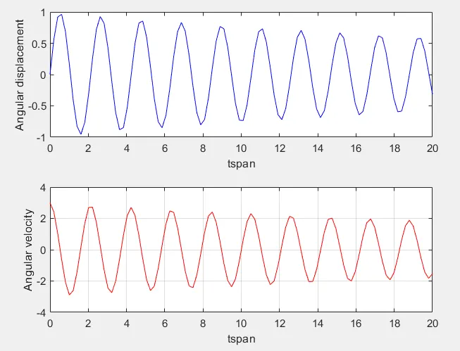
Output :

The output of the motion of simulation of simple pendulum between 0-20 sec, for angular displacement=0,angular velocity=3 rad/sec^2 at time t=0.

Youtube link of simulation video : https://youtu.be/sJkk3Qn8cuI