Week 3 - External flow simulation over an Ahmed body.

Objective :

In this challenge,

1. We will ,Describe Ahmed's body and its importance.

2. Explain the reason for the negative pressure in the wake region and show the vector plot clearly showing the wake region.

3. Explain the significance of the point of separation.

4. We will simulate the velocity and pressure contours of flow over Ahmed's body and we will validate the drag coefficient.

5. Finally, we will perform the grid independency test and provide the values of drag and lift with each case.

Introduction :

• External flows in general can be classified as flows over immersed bodies where flow features (such as boundary layers) around the body can develop freely without constraints of adjacent surfaces:
  ‐ Airflow over aircraft and ground vehicles
  ‐ Water flow over a submersible vessel
  ‐ Flying baseballs, footballs and golf balls
• One of the most important areas of interest in studying external flows are fluid forces acting on the body, as they define the dynamics of an object traveling through a fluid.
• Unlike internal flows which could be solved analytically for the entire range of laminar 𝑅𝑒, analytical solutions to flows over even simple shapes are only possible for very low Reynolds numbers 𝑅𝑒~1 which are of little interest in practical applications.
• Even at modest laminar regime numbers 𝑅𝑒~10, external flows start developing separation regions and wakes which cannot be described analytically.
• The boundary layer theory for laminar and turbulent flows provided us with relations and correlations which can clarify some, but not all, characteristics of external flows.
• An external flow is, indeed, a challenging problem even in present-day fluid dynamics.
• In external flow problems, the flow either moves over a stationary body (e.g., a wind tunnel experiment) or a body moves in a quiescent fluid (e.g., a flying airplane).
• In fluid dynamics it is common to describe the flow in the reference frame fixed to the body, i.e., fluid is flowing over a stationary body.
• Upstream conditions (velocity, pressure, density) are normally used as inputs to characterize the flow upstream of the body at a location where the flow is not affected by body’s presence. In most cases, constant upstream conditions are used.
• External flow characteristics depend greatly on a body’s shape.While there are many different possible shape variations, two extremes are:
  => Bulky shapes, like buses or large trucks:
  ‐ Flows are highly separated and unsteady, and steady-state approximation may not give accurate results.
  ‐ Boundary layers are significantly affected by flow separations, and the boundary layer theory is largely inapplicable.
  => Streamlined shapes like airplanes or submarines:
  ‐ Flows are attached over a significant part of the body surface.
  ‐ The boundary layer theory can be taken advantage of in certain cases.
  ‐ The steady-state assumption holds in many situations.
• The vast majority of practical external flows are turbulent in a sense that the flow is turbulent in a part of the domain around the flow.
• All turbulent external flows invariably have laminar regions, e.g., a boundary layer immediately after its onset or slow-moving separation regions.
• If laminar regions are very small compared to the turbulent region, then the flow can be assumed to be fully turbulent.
• On the other hand, if a laminar boundary layer persists over a significant portion of the surface, then both laminar and turbulent regimes must be included in the analysis.
• External flows develop whenever an object is moving through a fluid.
  ‐ Example – have you ever felt the air resistance while speeding up on your bike?
• As an object travels though the fluid, its dynamics are affected by pressure and viscous forces.
• Therefore, for external flow analysis, our primary objectives are prediction of fluid forces acting on the object and understanding the flow physics defining these forces.

Ahmed's body and its importance :

Optimized external car aerodynamics is necessary to achieve efficient vehicles with minimized fuel consumption, CO2 emissions, and noise, while keeping a good driving stability. Steadily increasing computer power has been raising the importance of simulating the external aerodynamics of vehicles and computing the corresponding aerodynamic characteristic numbers. At present, an efficient resource management gains increased importance everywhere. A substantial part of the development time of cars is therefore invested in optimization. This is possible only and particularly by virtual development. In order to establish such development processes in the car industry, reliable simulation models validated by experiments are needed. Model experiments suitable for providing validation data make use of model bodies with geometries characterized by variable parameters, such as the slant angle at the back. The flow region which presents the major contribution to a car’s drag, and which poses severe problems to numerical predictions and experimental studies as well, is the wake flow behind the car. The location at which the flow separates determines the size of the separation zone, and consequently the drag force. Clearly, a more exact simulation of the wake flow and of the separation process are essential for the correctness of drag predictions.However, a real-life automobile is a very complex shape to model or to study ,therefore experimentally one such body is the Ahmed body, a bluff model body of simple shape with basic aerodynamic properties of a vehicle, which has been used for many reference investigations.Ahmed body is a 3D model,Thatis representative of standard model of passenger car.The aim for this project is to develop, refine, and validate the latest generation of turbulence models for selected examples encountered in vehicle aerodynamics. The validation of turbulence models requires the availability of detailed experimental data.This is also used in valdating CFD codes.If you have your code before trusting it or validating your code you need to make sure that the results are comparable with the experiment data of Ahmed body.If it matches then you can trust your code and use your code to test for other geometry.This is a research model which was built in real life ,which many people made experimental analysis on it and we have a lot of rich data.So it can be very much useful in validating CFD codes.

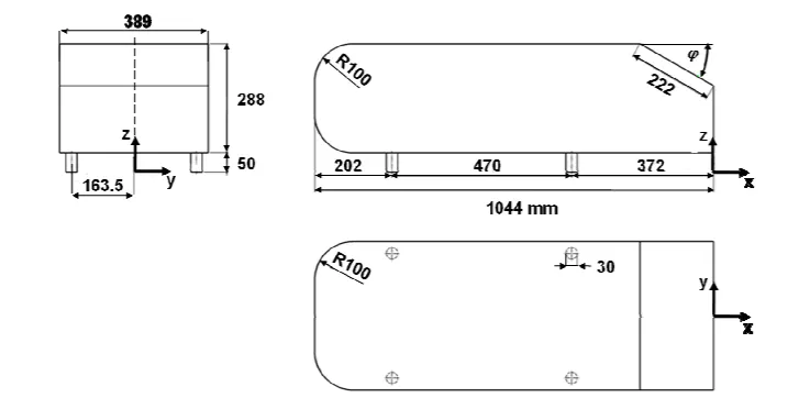
Geometry of the Ahmed body

Solution procedure :

• We will simulate the flow over Ahmed's body with the steady state case.Then for solving we follow the below procedure :

1)Creation of geometry

2)Meshing

3) Problem setup

4)Solving

5)Post processing

• Then while simulating the model, and we plot the coefficient of drag and lift plot and we show that the flow has converged and reached steady state.Then we will post process the results and also we find the drag coeffcient and compare them with experiment value.
• Then finally,we will discuss the effect of Reynolds number on the coefficient of drag.
• Finally, we will perform the grid independency test and provide the values of drag and lift with each case.

Simulating the flow with the Steady case :

In the ANSYS work bench we first open the fluent module by drag and drop.The we follow the procedure we have mentioned above

1) Geometry setup :

• In fluent module we have to open spaceClaim and import the geometry.

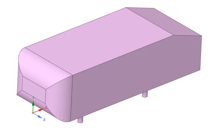
• Here as the body is perfectly symmetric, we can run the simulation by considering the only half body. This is the best practice where you can save on the number of cells and get the results faster as well.
• We use the split body command in spaceclaim which is under design to split the geometry it into two parts and delete the other part.

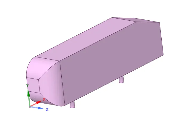
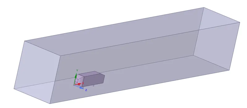
• Here we want to simulate the flow over Ahmed body i.e., we dont need the mesh inside Ahmed body.So we have to create a box or enclosure covering the model.We create this by using enclosure.
• To create enclousure select the geometry -> under prepare -> select enclosure then give dimensions by unchecking the symmetric dimensions so that we can have more control.
• In front we give 2m,back 5m and top 1m and bottom 0m and sides 0.5m each side.Then clicking okay spaceclaim automatically creates a single large volume enclosure of dimensions we gave by subtracting Ahmed body volume from it.

• Now we need to suppress the Ahmed body for physics because it may lead to creation of mesh for Ahmed body also which we dont want because the analysis is going to be over the Ahmed body so we dont need inside mesh,which needs lot of cells and computational power and eventually more time to solve .So we supress it for physics.
• Now we add a region of refinenment which is local refinemnt to capture the wake region exactly.The dimesions of region of refinement can be known if you run a base line simulation,so that you know the exact dimension of wake region and can captured perfectly.This is done by creating one more small enclosure in front the Ahmed body.
• Now for the second enclosure we give the dimensions as 0.5m in front,1m back side ,0.5 m on top,0m for bottom and 0.26m on both sides.This has to be done iteratively and changes from problem to problem.This is the reason we have to run a baseline setup.

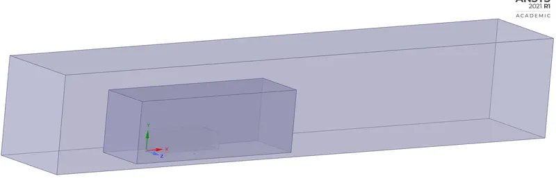
• Then when you click okay.you may see an error causing protruding bodies.When you mesh this you will see mesh overlap and the mesh in not going to connect perfectly.This causes because of two enclosure sharing a common area.So to get rid of this we have to do a interface check.If you do that by selecting interference you will see a huge interface.We will fix this by selecting prepare => Interference =>then click ok.You will see that it solves the problem and there is no overlap.
• Then in the left geometry structure if you see there will be two components one is the outer enclosure with which inner box has cut from it and other is the inner box with empty volume in the Ahmed body cut out .When these components are joined together that forms our flow domain.In order to all of this to work as one component we need to make sure that share topology is set to share.Only then these two individual blocks going to exchange information i.e., the meshing is going to be uniform and with perfect connectivity.
• Now if you open meshing and you will see that there is perfect mesh connectivity with no mesh overlap. This is the exact procedure you need to follow when you when you are performing an external simulation.The only things that changes from problem to problem is geometry and size of windtunnel.
• This completes the creation of geometry.Then we close the spaceClaim ,the progress will be saved automatically.

2) Meshing :

• For meshing we open Meshing,where we mesh our model so that we can use it to solve our model.
• We first select the entity by using the entity selection by using faces so that we can provide name for our entity selection.

steps : select the edge you want to name by using edge selection -> then press N -> name the selection.

• In the similar way we name our inlet,outlet,symmetry walls, bottom wall,Ahmed body as car wall.
• Then next thing to do is to mesh.We click the mesh option in the side window and create our base line mesh.We then refine mesh.Let's mesh the geometry .Once the mesh has done we need to see what are the things we have to refine.Let us refine one by one .

a) Method (Multizone method) :

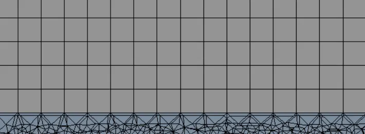
• Now comming to the refining mesh if you see out side the inner region there is a perfect structure made of straight lines i.e., no complex shape ,in 3D made of boxes.So when you have such a scenario like this it is better to use hexahederal mesh.Hexahederal meshes have the highest quality of all the mesh types so whenever it is possible it is better to use that.
• So to do this ,we right click mesh => insert =>insert => method =>in geometry - select outermost body => Apply for method - multizone(Whenever you use multizone it creates hexa meshes wherever it is possible and in another regions where it is having different mesh tyoe it is going to have perfect connectivity)
• For main global mesh let us give mesh size of 100mm and in that give maximum size as 100mm so that we can evenly sized mesh in the outer region.If you generate mesh you will see nice boxes or hexahederal mesh which nicely connects with inner tetrahederal mesh perfectly.

b) Sizing(Body sizing) :

• We are making the mesh inside the small enclosure finer by using sizing.To do this,
• Right click on mesh => sizing => in geometry -we select inner box or enclosure and give size 40mm => Then generate mesh again you will see inner enclosure is refined finer.

c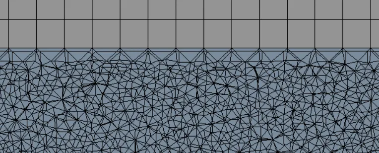

c)Sizing(Edge Sizing) :

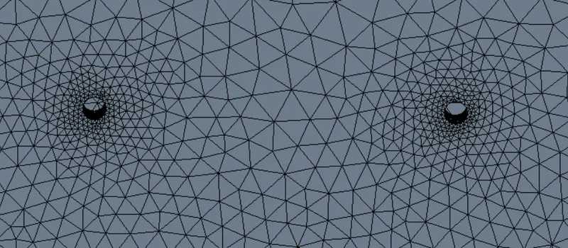
• If you see that the cylinder pillars are approximated as polygons because element size is quite big over there.
• To fix this we we select only those faces by single select tool and give a mesh size of 5mm and generate mesh,now you will see that they are much better than before and can be seen as cylinderical pillars.

d) Sizing(Body sizing) :

• Now we are making the mesh size of Ahmed body finer by using sizing.To do this,
• Right click on mesh => sizing => in geometry -we select Ahmed body and give size 20mm => Then generate mesh again you will see Ahmed body boundary faces is refined finer.

e) Inflation :

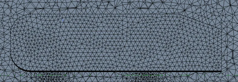
• Inflation layer helps us to create a body fitted mesh.It means it creates a layer of mesh same as the geometry around the Ahmed body .
• Since the flow around the Ahmed body is very important we need to take that region and create inflation layers so that flow is captured exactly.
• To do this we have to right click on mesh => sizing => in geometry - we select small enclosure and for boundary - we select Ahmed body boundary layer.
• And for inflation option we use first layer thickness and we give this based on y+ value and the turbulence model we use.Here we use k-omega SST turbulence model so y+ should be in between 0.1 to 5.Lets calculate the first layer thickness.

1. U∞ = freestream velocity = 25 m/s
2. ρ = freestream density = 1.225 kg/m3
3. μ = dynamic viscosity = 0.000017894 kg/m s
4. L = length of Ahmed body(m) = Rex=ρU∞Lμ">1.044 m
5. desired y+ = 1

=> Then Reynolds number, Re = (ρ*U∞*L)/μ = (1.225*25*1.044)/ 0.000017894 =1786772.1023806867

=> skin friction coefficient, C_f = (0.026)/Re ^1/7 = 0.026/(1786772.1023806867)^1/7 = 0.00332522173

=> wall shear stress, Tau_wall = (C_f*ρ*U∞^2)/2 = (0.00332522173*1.225*(25)^2)/2 =1.27293644352

=> friction velocity , U_friction = (Tau_wall/ρ)^1/2 = (1.27293644352/1.225)^1/2 = 1.01937813918

=> Therefore, first layer thickness , Δs = (y+ * μ)/(U_friction*ρ) = (1*0.000017894)/(1.01937813918*1.225) = 0.00001432966 m = 0.01432966 mm

• Now we got the first layer thickness ,let us give the above first layer thickness and maximum of 10 growth layers and with a growth ratio of 1.2 for inflation layers.

• Clear the generated data and we have to mesh again.By this we have completed the meshing process then we have to update or generate the mesh again.You can observe formation of inflation layers.

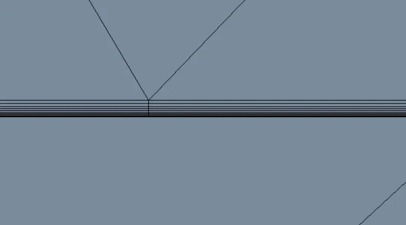
• Below is the sectional view of the final mesh.

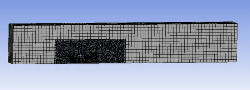
• Now we have to check the quality of the mesh.steps : mesh ->quality-> mesh metric-> Element quality

• Here our minimum quality is around 17 %,so we can move further for our solution setup.

3) Problem Setup :

• To set up our problem we open Fluent and setup inital conditions , boundary conditions material etc.,
• We first start with checking the mesh quality using perform mesh check under domain.If no error is seen in console window then we can proceed further.
• Then we move move to setting up physics where we select the solver ,viscous model ,initial and boundary conditions etc.,
• We use a steady state pressure based solver to solve our model.

Physics :

General :

Solver type : pressure based

time : steady state

velocity formulation : absolute

models :

viscous model : k-omega SST

Material : Air

Zones :

Cell zone : you will see our volume zone which is basically our internal volume basically mesh, and it is of type fluid.

Boundary conditions :We will basically give our boundary conditions here such as inlet velocity and outlet conditions.

we give,

Inlet :

velocity : 25 m/sec

Outlet :

pressure outlet : gauge pressure = 0 pa

Car walls :

wall : No slip

Symmetry walls :

type : symmetry

Bottom wall :

type : wall - No slip

• Now we are almost ready to run the simulation ,but as the solution is being solved we want to moniter different flow quantities while the solution is being generated ,we use definitions for this.But before that we have to initialize the domain.We use the Hybrid initialization , this provides a very good initial condition .
• Then we go to postprocessing or results and we need to create a cut plane to see how the velocity and pressure vary over Ahmed body look like.This is something we want to moniter as the simulation is running.We can see flow going through X - axis .So, we have to create a plane which has normal in the Z - direction.

steps : In results -> create -> plane -> select point and normal -> give values - point =(0,0,0) and normal along Z - axis (0,0,1) -> name it as cut plane -Z .

• Now we want to see the pressure and velocity contour.
• For contour -> go to solutions tab -> graphics -> contour -> in contour of : select velocity under that velocity magnitude -> select cut plane -Z and press save /display.
• Then you can see the initial values for velcity which is obtained by initialization which is not the final one.
• In the same way create the pressure contour plot also.
• Then we want to create animation so that we can see how these parameters are varying when problem is being solved.
• For that,

steps : Activities -> solution animation -> select velocity contour which we have created -> preview -> set the required view and use active -> and name it as velocit animation.

• In the same way create the animation for pressure contour plot also.
• Now we also want to moniter the lift and drag coefficient plot of Ahmed body while the solution is being run.Create lift and drag coeffcients plots.

steps : Definitions -> New -> select the force report -> drag -> select cylinder wall under zones -> check report file and report plot -> then okay.

• In the same way create a plot for lift coefficient also.

• In solution method we use SIMPLE .

4) Solving :

• Give iterations such that your solution is converged.
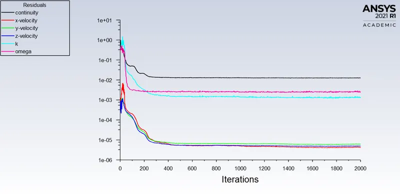
• Run the simulation until the steady state is reached.Lets run for 2000 iterations ,we can find the solution is converged.
• Then we can see that in the residual plot that residuals dropping and reach a steady state after 450 iterations.
• .Then post process the results.

5)Post processing :

Residuals plot :

• You can observe from the below plot the residuals has converged after 450 iterations.

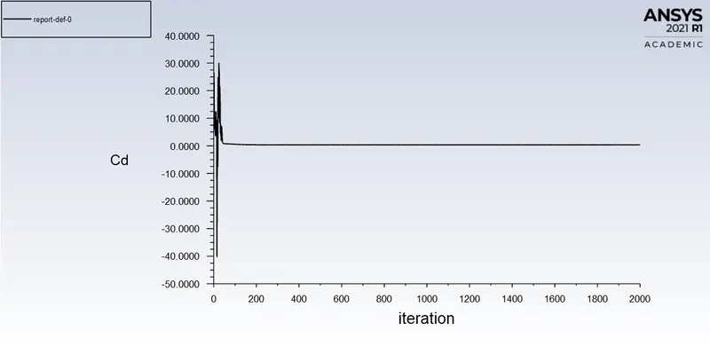
Drag plot :

• You can observe from the below plot that drag coefficient has reached the steady state as it follows the same pattern after 50 iterations.

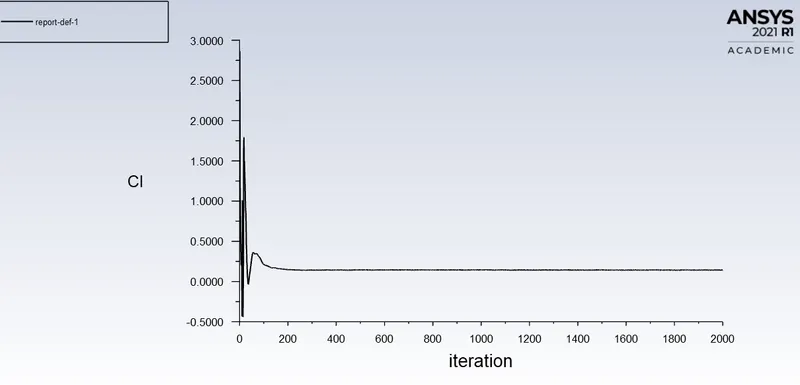
Lift plot :

• You can observe from the below plot that lift coefficient has reached the steady state as it follows the same pattern after 200 iterations.So we can conclude that the flow has converged.

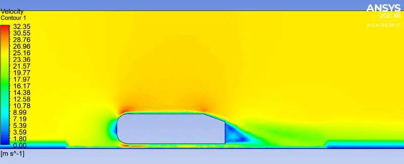
Velocity contour :

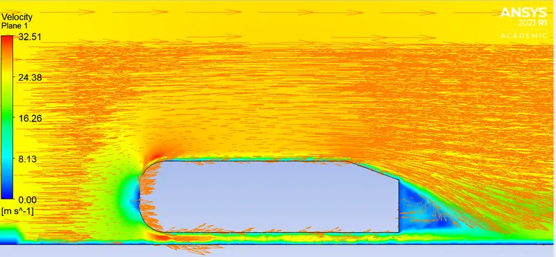
• The below plot is the velocity contour you can see the formation of wake behind of Ahmed body.

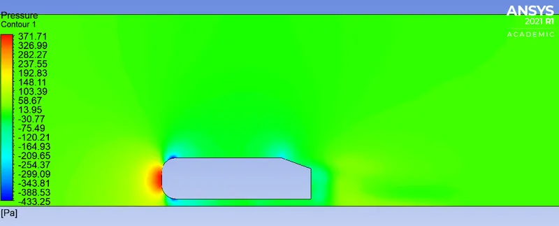
Pressure contour :

• The below plot is the pressure contour of flow over Ahmed body.

Vector plot :

• Here in the below vector plot you can see that formation of wake.In that wake you can see the vectors recirculating in the wake region which means flow is recirculating in the wake.

Boundary Layer Separation :

• In general, wall-bounded flows are subject to pressure variations due to surface curvature or an external forcing.
• When the freestream pressure increases in the direction of flow, it is known as an adverse pressure gradient.
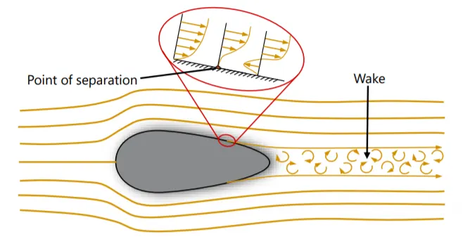
• Adverse pressure gradients cause the flow to slow down. When the velocity gradient at the wall approaches zero, the flow will lift off the surface, diverting the streamlines away from the wall. This process is known as separation.
• When a boundary layer becomes separated, the boundary layer equations are no longer valid. However, we can predict the point of separation by monitoring the velocity gradient (or shear stress) at the wall in our solution and noting where it becomes close to zero.
• The pressure field in the fluid flow past an object is nonuniform. When the pressure gradient is nonzero, the velocity profile is affected .
• Separation of boundary layers in general occurs when the velocity of the boundary layer “struggling” against an adverse pressure gradient becomes nearly zero, i.e, pressure increases as the wall fade away this pushes the fluid back .If the momentum of fluid is insufficient the fluid reverses its direction and seperates from the wall.
• The separation point is defined as a location between forward and inverse flow where the wall shear stress is zero.
• The thickness of the boundary layer abruptly increases at the separation point, and the layer is forced off the surface by the reversed flow near the wall.
• Detached flow takes the form of vortical structures, which can be laminar or turbulent depending on the flow regimes.

Significance of the point of separation :

• In our case we can easily understood that ,at sharp corners and turns the flow naturally separates, as can be easily understood from the conservation of momentum.
• This effect is same as flow in a backward step problem.

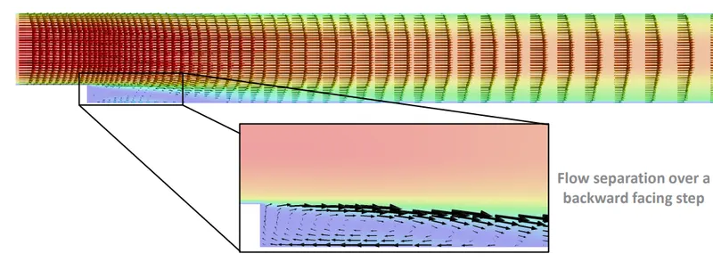
• At the corner, the boundary layer maintains its momentum in the direction of the flow, and simply cannot stay attached in the absence of an external pressure gradient forcing it to turn around the corner.
• So as the flow tends to go straight then due to this it forms a low pressure region at that point and back of ahmed body.Then this low pressure sucks the flow which is going straight and forms a recirculation zone.
• And then finally you can see that this leads to the recirculation zone and formation of large wake backside of the Ahmed body.You can see the formation of wake in the velocity contour.

Reason for the negative pressure in the wake region :

• As we know that ,at sharp corners and turns the flow naturally separates, as can be easily understood from the conservation of momentum.
• At the corner, the boundary layer maintains its momentum in the direction of the flow, and simply cannot stay attached in the absence of an external pressure gradient forcing it to turn around the corner.
• So as the flow tends to go straight then due to this it forms a low pressure region at that point and back of ahmed body.Then this low pressure sucks the flow which is going straight and forms a recirculation zone and formation of large wake backside of the Ahmed body.This also leads to formation of large wake.
• You can see the formation of wake in the velocity contour and if you see in pressur contour in wake region you will see negative pressure.Actually it is not the negative pressure it is just the low pressure region.As we have taken with reference to 0 guage pressure you can see the negative values.If you change the outlet gauge pressure or done the simulation by taking absolute pressure you will not any negative values but it will lead to round off errors as the flow is incompressible there will small pressure variations.So it is better to use 0 gauge as reference for simulations of incompressible flow.

Grid independency test and effect of grid size on values of drag and lift :

• Let us perform grid independency test and tabulate all the values of drag and lift with each case i.e., with each grid size and compare with the coefficent of drag value of experimental value i.e., 0.33.

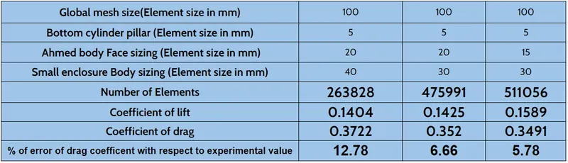
• In the above table we can observe that as we are refining the mesh we can see that we are getting closer to the experimental value of drag coeffcient and the % of error is decreasing.
• We can also observe that almost all the values are equal but there is a difference in the range of 1e-2.
• So,it is better to use small mesh size but the thing is with the decrease in the grid size there will be increase in computational effort.
• So the results which we got are very much satisfactory and very close to the Experimental value.
• So, we can conclude that our result is grid dependent.

Animation :