Week 1- Mixing Tee

Objective :In this challenge ,we will simulate a mixing tee by setting up steady-state simulation to compare the mixing effectiveness when hot inlet temperature is 36°C & the Cold inlet is at 19°C .We will perform the simulation for different cases i.e, for short and long mixing tee with different momentun ratios.We will first use the k-epsilon and k-omega SST model for the first case and judge which is best suited for model for our case by comparing it with the analytical solution and use the best one for our further cases.Then after simulating the model then we will post process the results by using cut planes and line plots and plotting velocity and temperature contour on them  along and across the pipe.Then we perform Mesh independent study and finally we will discuss the effect of length and momentum ratio on results.

Introduction :We can find Mixed tee in lot of places including our home. Mixing tees are widely used in the petrochemical industry, in which two fluid streams with different physical and/or chemical properties mix together.It is T- joint and are important flow control devices.It is called T- joint because it splits the flow and angle between them is 90°.

                                               

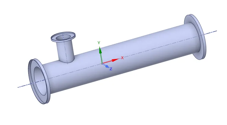
Here in our case we use the working fluid as air where we use hot inlet temperature 36°C in the x-direction & the Cold inlet at 19°C from y direction inlet having different inlet velocities .Air from both the inlets mixes and comes out from the outlet with desired temperature.

                                         Momentum ratio = velocity at cold inlet / velocity at hot inlet

Solution procedure :

• Firstly let us start by taking the case of short tee with momentum ratio 3 and compute it with k-epsilon and k- omega SST viscous model 
• Then for solving we follow the below procedure :   

                 1)Refining the geometry 

                 2)Meshing

                 3) Problem setup

                 4)Solving

                 5)Post processing

• Then after simulating the model then we will post process the results and take the required results  to compare between them and with analytical solution.
• We find the analytical solution and compare it with above values genrated by different viscous model and pick the best one for our case and use the same viscous model for the rest of the cases.
• Then for the remaining cases we use the above select model and we follow the same procedure for simulating the other cases.
• Then we perform Mesh independent study
• We then,in a table, compare the following values from the cases. 
  1. Cell count
  2. Average outlet temperature
  3. Number of iterations for convergence
• Finally we will discuss the effect of length and momentum ratio on results.

Simulation of short mixing tee with momemtum ratio 3 with k - epsilon viscous model :

In the ANSYS work bench we first open the fluent module by drag and drop.The we follow the procedure we have mentioned above

1) Refining the geometry :

• IN fluent module we have spaceClaim.We first load the cad model to clean up and refine it so that we can use it for simulation.
• In the model you can see the thickness.These will be useful to do a solid simulation,for example to find the heat transfer to surroundings from fluids etc,.Which is not required in our case as we are intrested in flow simulation we dont extra parts.
• We need only fluid volume which are the parts our fluid is going to interact,here in our case inside part.
• We use volume extraction to get the fluid volume in spaceClaim.

                    steps : prepare -> volume extract -> select the fluid volume by selecting the edges -> Then ok.

• Then new object will be added to the tree.Then hide the solid volume and the left is fluid volume which we generated.
•                                        
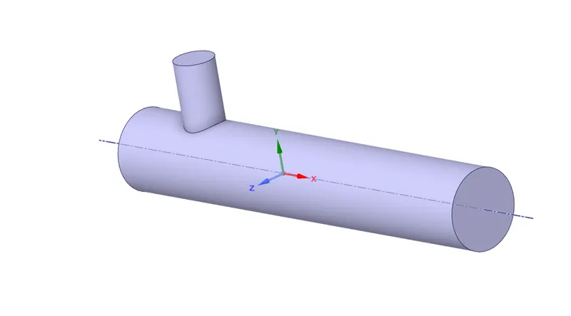
• We supress the solid volume by using supress for physics such that  it is not involved in the mesh generation and solution process.
• Then close the spaceClaim ,the progress will be saved automatically.

2) Meshing :

• For meshing we open Meshing ,where we mesh our model so that we can use it to solve our model.
• We first select the entity by using the entity selection by using faces so that we can provide name for our entity selection.

        steps : select the face you want to name  by using face selection (CTRL + F) -> then press N -> name the selection.

• In the similar way we name our inlet,outlet,walls.
• Then next thing to do is to mesh.We click the mesh option in the side window and then under defaults you will find element size,there give the element size as required.Here we use 0.003,which can give the satisfactory results.
• Then we check the element quality.You should have minimum quality of 5%(0.5).

        steps : mesh ->quality-> mesh metric-> Element quality

                                      

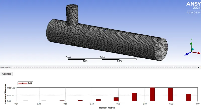
• Here our minimum quality is around 35% ,so we can move further for our solution setup.

3) Problem Setup :

• To set up our problem we open Fluent and setup inital conditions , boundary conditions material etc.,
• We first start with checking the mesh quality using perform mesh check under domain.If no error is seen in console window then we can proceed further.
• Then we move move to setting up physics where we select the solver ,viscous model ,initial and boundary conditions etc.,
• We use a steady state pressure based solver to solver our model.

Physics :

General :

                     Solver type      :      pressure based

                         time            :      steady state

      velocity formulation         :       absolute

• Then we select the k - epsilon realizable model which is upgraded version of k -epsilon model with standard wall functions.Here we have to selecct the energy equation as we are solving for the temperature.

models  :

                      viscous model  :        k-epsilon

                        type             :       realizable 

            Near wall treatment   :       standard wall functions

• Here we use air as our working fluid.

Material  :

                       name           :       air

Zones :

                  Cell zone :  you will see our volume zone which is basically our internal volume basically mesh, and it is of type fluid.You can also change material name here if required.

  Boundary conditions :We will basically give our boundary conditions here such as inlet velocity and temperature and outlet conditions.

                       given our  inlet x velocity =3 m/sec and momentum ratio = 2 then ,  

                       Momentum ratio = velocity at cold inlet(y) / velocity at hot inlet(x),

                       => velocity at cold inlet(y) = 3*2 = 6m/sec 

   inlet -x :  

                      velocity        :      3 m/sec

                 Temperature     :     36 °C

   inlet -y :  

                         velocity     :    6 m/sec

                  Temperature    :    19 °C

 outlet  :

      pressure outlet : gauge pressure = 0 pa

• Now we are almost ready to run the simulation ,but as the solution is being solved we want to moniter some physical quantity during the run time ,here we need to moniter the outlet temperature.

        steps :  solution -> under definitions -> select new -> select the surface report ->area weighted average-> and select the parameter you want to moniter-> check report file and report plot ->then okay.

• Here we will moniter temperature and standard deviation of temperature at the outlet ,which is used to know the mixing effectiveness its low value is equal to very good mixing.

          steps :  solution -> under definitions -> select new -> select the surface report ->standard deviation->temperature at outlet -> check report file and report plot ->then okay.

• Finally after the setting up of initial conditions and boundary conditions the next thing to do is initialization.

Initialization :

When performing CFD analysis  ,as we are solving for pressure and velocity and temperature and other variables we need to providde starting values for all these variable at all cells at t=0.

        steps : solve -> initialization -> Hybrid -> initialize (t=0) 

• The next thing to do is run by clicking calculate.We run for 500 iterations 
• Then we can see that in the residual plot we see residuals dropping and reach a steady state after 175 iterations.

                                     

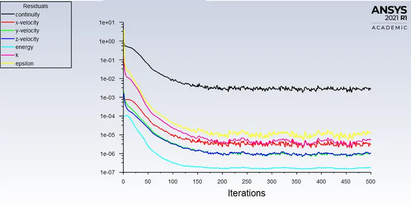
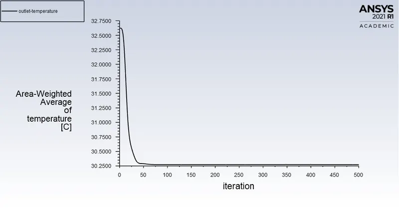
• In the report of average outlet temperature you will see the temperature is 30.30 °C which almost steady after 75 iterations   

                                     

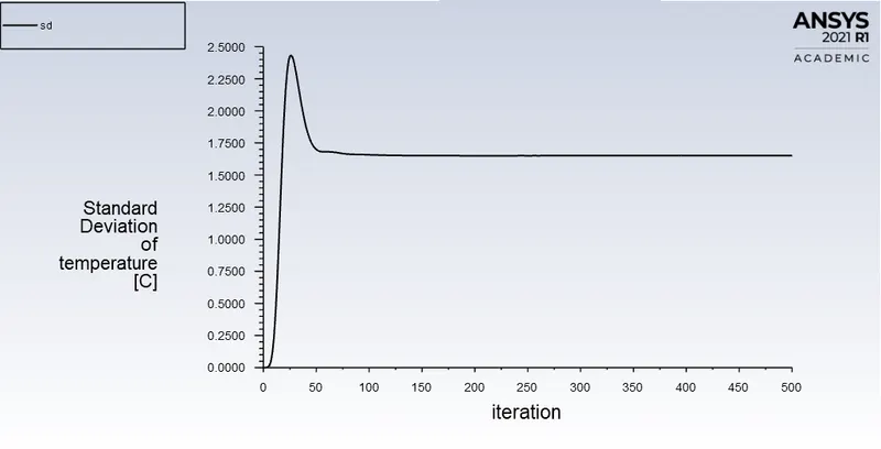
• In the report of standard deviation of  temperature at the outlet you will see it is 1.650 which almost steady after 75 iterations.

                                     

Simulation of short mixing tee with momemtum ratio 3 with k - omega viscous model :

• Now lets run the same simulation with same initial and boundary conditions by using k-omega SST model to see which one is best suited for our model with less computaional effort and satisfied accurate solution.
• Initial meshing and setup is same as the previous one but in the viscous model we use k-omega SST model.

• Physics :

  General :

                       Solver type      :      pressure based

                           time            :      steady state

        velocity formulation         :       absolute

  • Then we select the k - omega SST model which is upgraded version of k -omega model .Here we have to selecct the energy equation as we are solving for the temperature.

  models  :

                 viscous model        :         k-omega

                         type             :          SST

  • Here we use air as our working fluid.

  Material  :

                         name           :         air

  Zones :

                    Cell zone :  you will see our volume zone which is basically our internal volume basically mesh, and it is of type fluid.You can also change material name here if required.

    Boundary conditions :We will basically give our boundary conditions here such as inlet velocity and temperature and outlet conditions.

                         given our  inlet x velocity =3 m/sec and momentum ratio = 2 then ,  

                         Momentum ratio = velocity at cold inlet(y) / velocity at hot inlet(x),

                        =>  velocity at cold inlet(y) = 3*2 = 6m/sec 

     inlet -x :  

                           velocity    :     3 m/sec

                    Temperature   :      36 °C

     inlet -y :  

                         velocity     :     6 m/sec

                   Temperature   :     19 °C

   outlet  :

             pressure outlet     :   gauge pressure = 0 pa

  • Now we are almost ready to run the simulation ,but as the solution is being solved we want to moniter some physical quantity during the run time ,here we need to moniter the outlet temperature.

          steps :  solution -> under definitions -> select new -> select the surface report ->area weighted average-> and select the parameter you want to moniter-> check report file and report plot ->then okay.

  • Here we will moniter temperature and standard deviation of temperature at the outlet ,which is used to know the mixing effectiveness its low value is equal to very good mixing.

            steps :  solution -> under definitions -> select new -> select the surface report ->standard deviation->temperature at outlet -> check report file and report plot ->then okay.

  • Finally after the setting up of initial conditions and boundary conditions the next thing to do is initialization.

  Initialization :

  When performing CFD analysis  ,as we are solving for pressure and velocity and temperature and other variables we need to providde starting values for all these variable at all cells at t=0.

          steps : solve -> initialization -> Hybrid -> initialize (t=0) 

  • The next thing to do is run by clicking calculate.We run for 500 iterations 
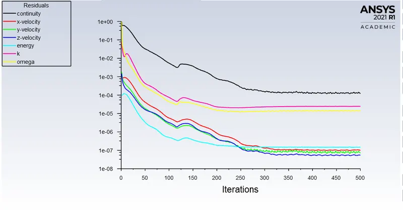
  • Then we can see that in the residual plot we see residuals dropping and reach a steady state after 290 iterations.

                                      

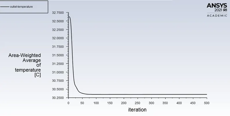
  • In the report of average outlet temperature you will see the temperature is 30.29 °C which is almost steady after 75 iterations   

                                      

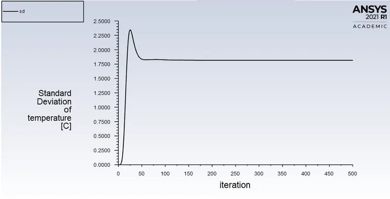
  • In the report of standard deviation of  temperature at the outlet you will see it is 1.815 which almost steady after 75 iterations.

                                      

Analytical Value :

• Now lets find the analytical solution so that we can use this value and compare with our numerical solution to judge the best model for our case.

                                                 

• First lets find all the parameters in the equation.

               Hot inlet :

                          density of hot air (rho_hot)        =      1.225 kg/m^3

                            volume of hot inlet (V_hot)      =       0.00267 m^3

                                 mass of hot air(m_hot)       =       rho_hot * V_h =1.225*0.00267= 0.003270 kg

         temperature of air from hot inlet(T_hot)       =       36 °C

            cold inlet :

                          density of cold air (rho_cold)       =      1.225 kg/m^3

                           volume of cold inlet (V_cold)      =       0.00132 m^3

                               mass of cold air(m_cold)       =       rho_cold * V_cold =1.225*0.00132= 0.001617 kg

        temperature of air from cold inlet(T_cold)      =       19 °C

• Now we have all the values lets substitute in the above formula to get analytical value

                                                          

                                                                

Comparision between the viscous models :

• We can see from the above results that the temperature obtained by k-epsilon model, 30.30°C is very close to the analytical value,30.375°C that obtained from k-omega SST model,30.29 °C.
• The standard deviation value for k-epsilon,1.650 , which is is quite low than k-omega SST,1.815.Which means the mixing has been quite better in k-epsilon than k-omega model.
• K-epsilon took just 175 iterations to reach steady state where as k-omega SST took 290 iterations ,which means higher computational effort for k-omega SST model.
• Finally we can conclude that from the above results that both the models are able to give the approximate closer value .Let us use k-epsilon turbulence model as it has given very near value to the analytical solution ,so the error percent will also be less.So,we perform our remaining cases with k - epsilon realizable model.

Case 1  :   a) Short mixing tee with a hot inlet velocity of 3m/s and Momentum ratio of 2 :

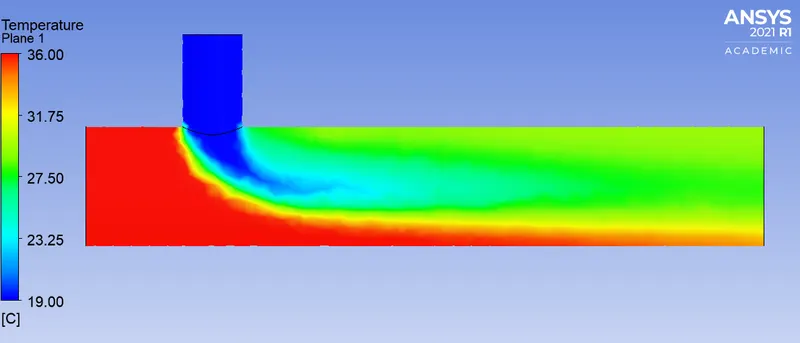
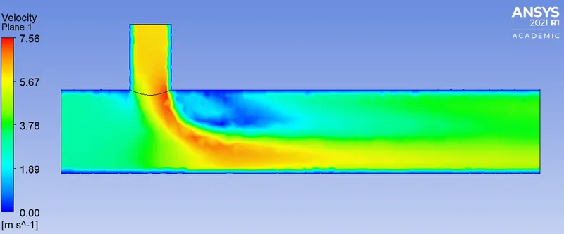
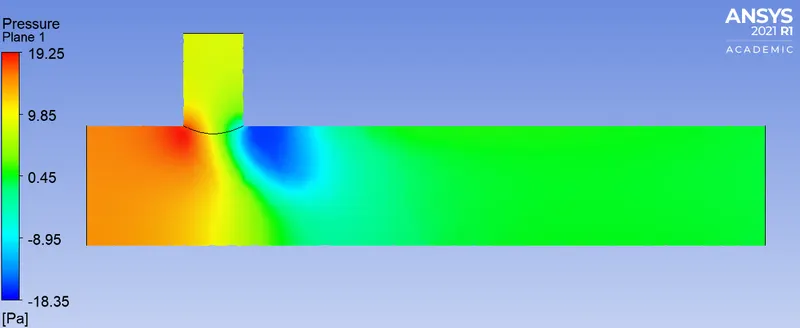
• As this is the case which we have performed above, so lets post process the results which we obtained by using k-epsilon realizable model.
• Contour of Temperature distribution on a plane along the length of tee.

                                      

• Contour of velocity distribution on a plane along the length of tee.

                                     

• Contour of pressure distribution on a plane along the length of tee.

                                    

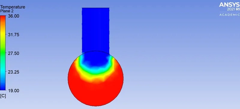
• Temperature distribution on a plane across the tee at the cross section where fluid from two inlets meet.

                                   

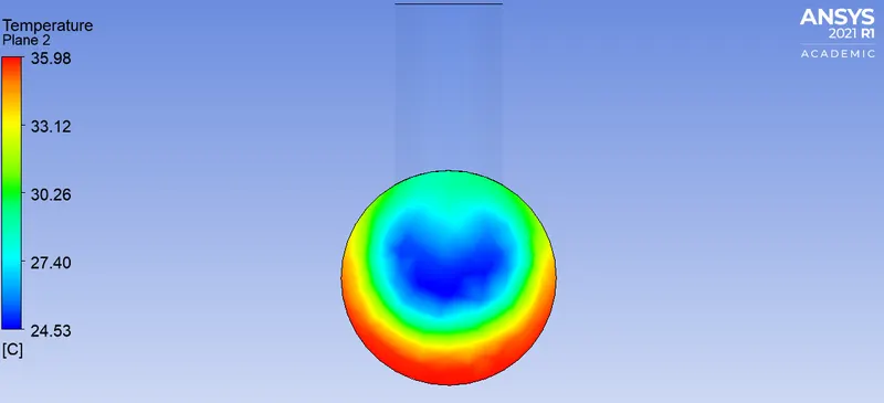
• Temperature distribution on a plane across the tee at the center of mixed tee. 

                                  

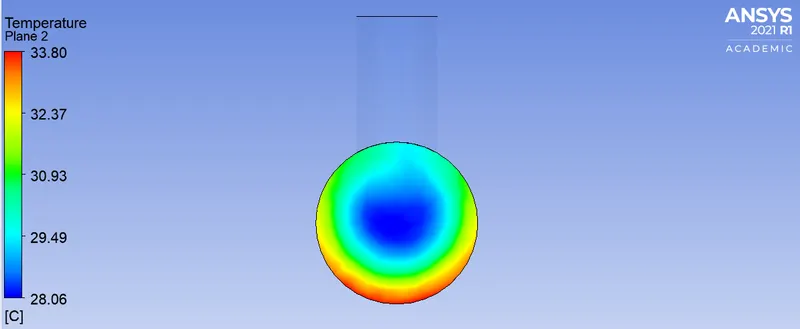
• Temperature distribution on a plane across the tee at the outlet of mixed tee. 

                                 

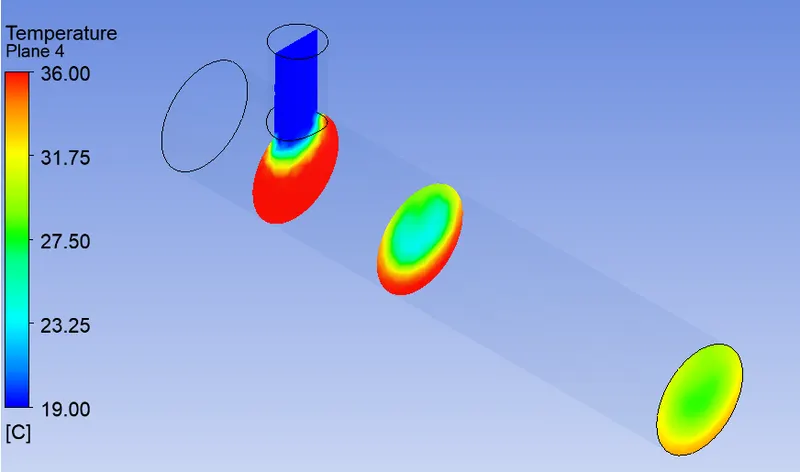
• Isometric view of temperature distribution on planes across the tee at different locations of tee. 

                                

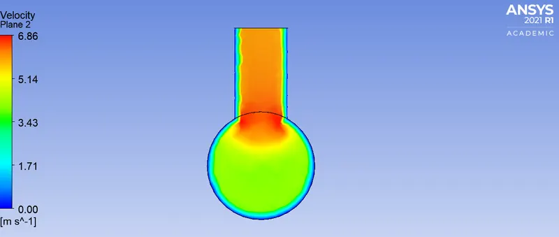
• Velocity distribution on a plane across the tee at the cross section where fluid from two inlets meet.

                                

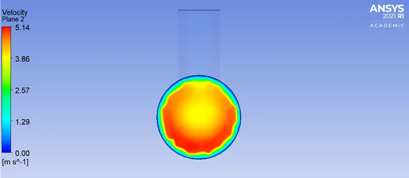
• Velocity distribution on a plane across the tee at the outlet of mixed tee. 

                                

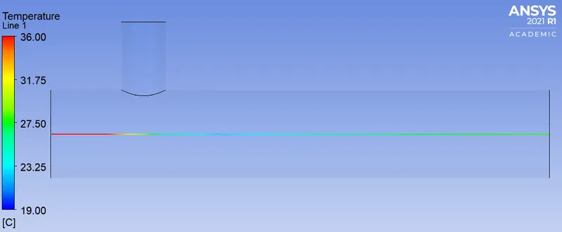
• Temperature distribution on a line plot along the length of tee.

                                

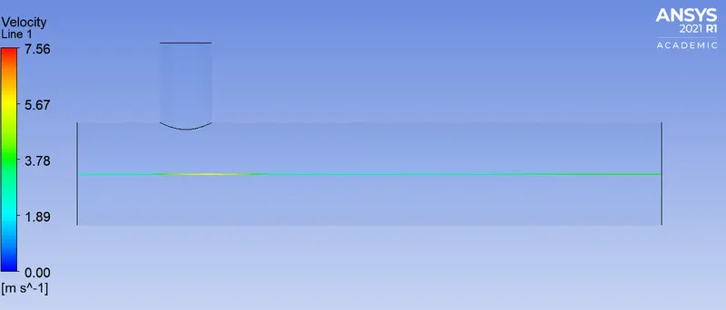
• Velocity distribution on a line plot along the length of tee.         

                               

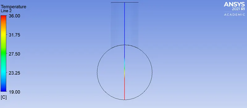
• Temperature distribution on a line plot across the length of tee at the cross section where fluid from two inlets meet.

                              

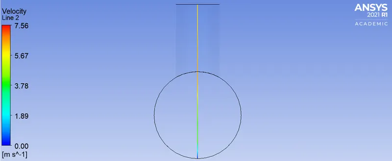
• Velocity distribution on a line plot across the length of tee at the cross section where fluid from two inlets meet.

                             

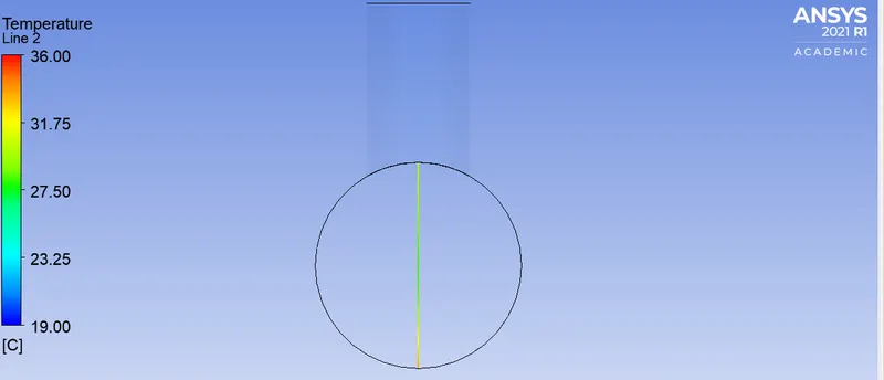
• Temperature distribution on a line plot across the length of tee at the outlet.

                             

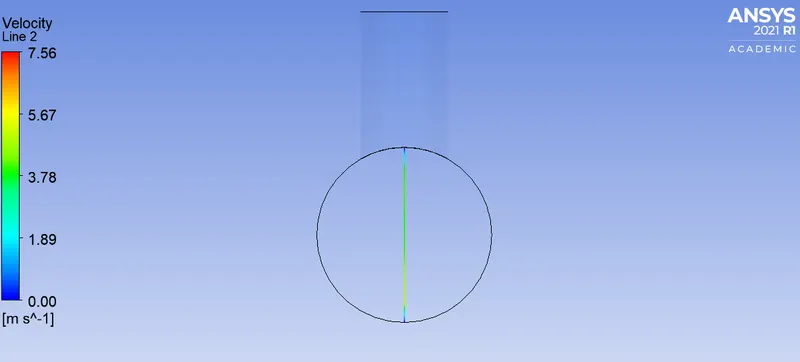
• Velocity distribution on a line plot across the length of tee at the outlet.

                             

b) Short mixing tee with a hot inlet velocity of 3m/s and Momentum ratio of 4 :

• We will follow the same process but we will have a different inlet velocity in y-direction as our momentum ratio changed.
• First we start with setting up physics where we select the solver ,viscous model ,initial and boundary conditions etc.,We use a steady state pressure based solver to solver our model.

Physics :

General :

                     Solver type      :      pressure based

                         time            :      steady state

      velocity formulation         :       absolute

• Then we select the k - epsilon realizable model which is upgraded version of k- epsilon model with standard wall functions.Here we have to select the energy equation as we are solving for the temperature.

models  :

                      viscous model  :      k - epsilon

                        type             :       realizable 

            Near wall treatment   :       standard wall functions

• Here we use air as our working fluid.

Material  :

                       name           :       air

Zones :

                  Cell zone :  you will see our volume zone which is basically our internal volume basically mesh, and it is of type fluid.

  Boundary conditions :We will basically give our boundary conditions here such as inlet velocity and temperature and outlet conditions.

                       given our  inlet x velocity =3 m/sec and momentum ratio = 4 then ,  

                       Momentum ratio = velocity at cold inlet(y) / velocity at hot inlet(x),

                      =>  velocity at cold inlet(y) = 3*4 = 12m/sec 

   inlet -x :  

                      velocity      :      3 m/sec

               Temperature     :     36 °C

   inlet -y :  

                      velocity     :    12 m/sec

               Temperature    :    19 °C

 outlet  :

      pressure outlet : gauge pressure = 0 pa

• Now we are almost ready to run the simulation ,but as the solution is being solved we want to moniter some physical quantity during the run time ,here we need to moniter the outlet temperature.

        steps :  solution -> under definitions -> select new -> select the surface report ->area weighted average-> and select the parameter you want to moniter-> check report file and report plot ->then okay.

• Here we will moniter temperature and standard deviation of temperature at the outlet ,which is used to know the mixing effectiveness its low value is equal to very good mixing.

          steps :  solution -> under definitions -> select new -> select the surface report ->standard deviation->temperature at outlet -> check report file and report plot ->then okay.

• Finally after the setting up of initial conditions and boundary conditions the next thing to do is initialization.

Initialization :

When performing CFD analysis  ,as we are solving for pressure and velocity and temperature and other variables we need to providde starting values for all these variable at all cells at t=0.

        steps : solve -> initialization -> Hybrid -> initialize (t=0) 

• The next thing to do is run by clicking calculate.We run for 333 iterations 
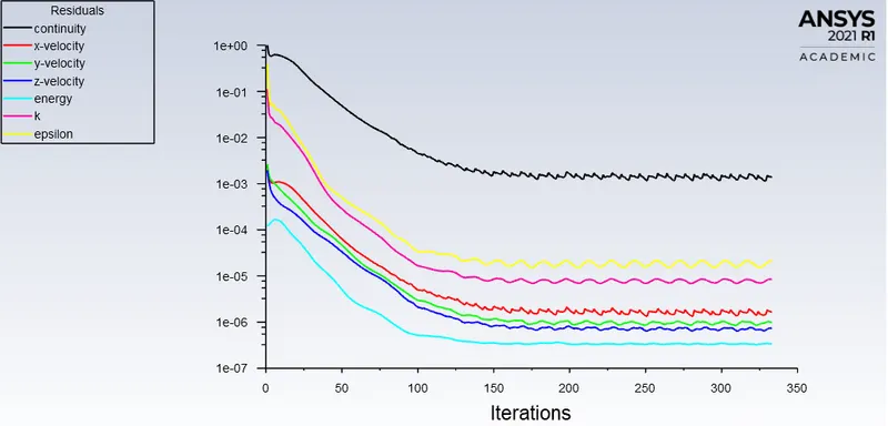
• Then we can see that in the residual plot we see residuals dropping and reach a steady state after 160 iterations.

                             

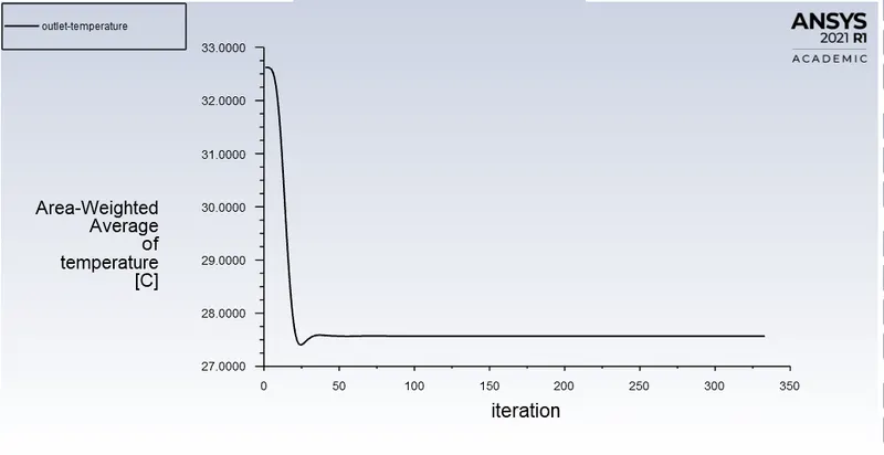
• In the report of average outlet temperature you will see the temperature is 27.56 °C which almost steady after 50 iterations   

                             

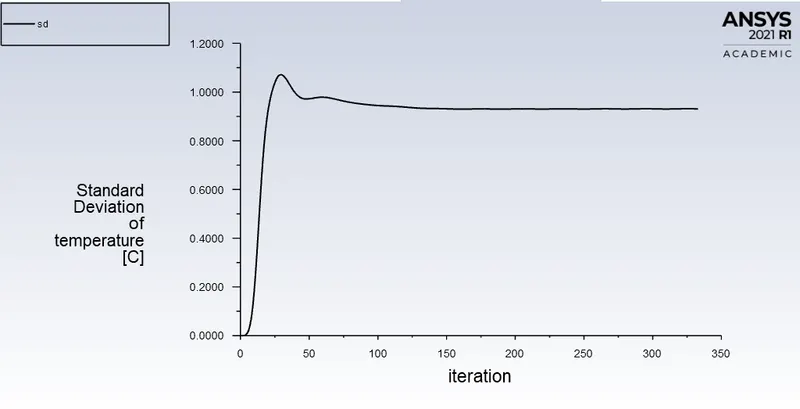
• In the report of standard deviation of  temperature at the outlet you will see it is 0.93 which almost steady after 120 iterations.

                              

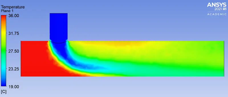
• Now, lets post process the results which we obtained by the above simulation.
  • Contour of Temperature distribution on a plane along the length of tee.

                              

• Contour of velocity distribution on a plane along the length of tee.

                              

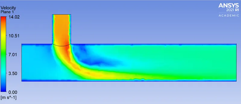
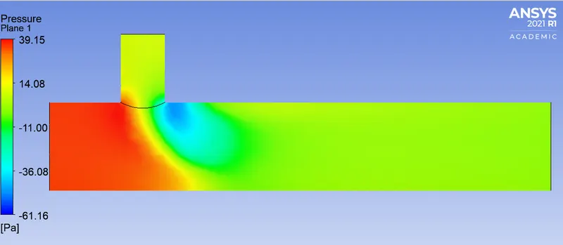
• Contour of pressure distribution on a plane along the length of tee.

                              

• Velocity vector distribution on pressure contour.

                              

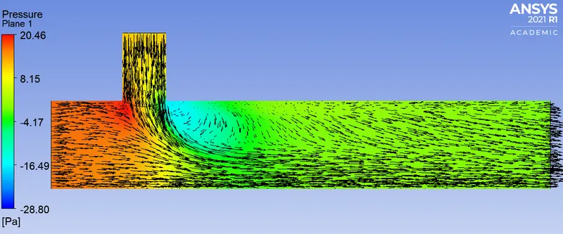
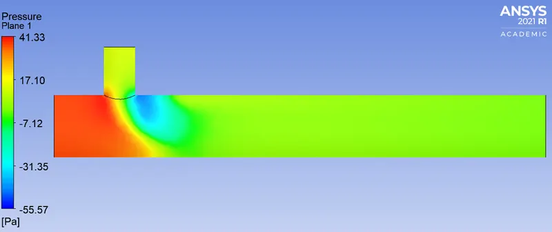
• You can observe a low pressure region beside the inlet of y-direction in the above figure, this is because when two fluids move from different ends a vacuum effect is created at that area ,this is because the air from y directions stops air from x-direction to enter that area and air from y direction also will not enter that area because the fluid in y- direction has high inertia  where area expands,  and will tend to move straight instead of directly entering that area.Then as this is low pressure region the fluid of high pressure tends to enter this area and recirculate.This happens in all the cases.

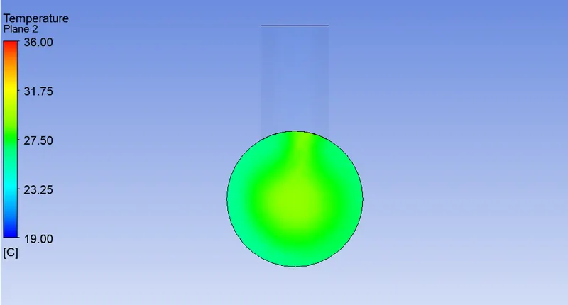
• Temperature distribution on a plane across the tee at the cross section where fluid from two inlets meet.

                              

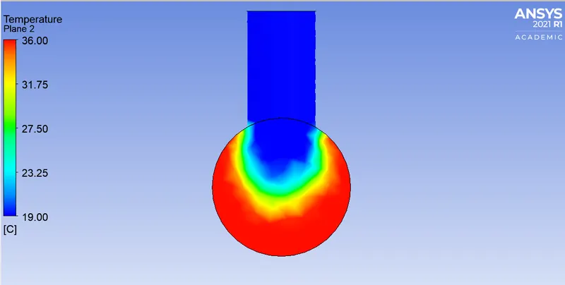
• Temperature distribution on a plane across the tee at the outlet of mixed tee. 

                            

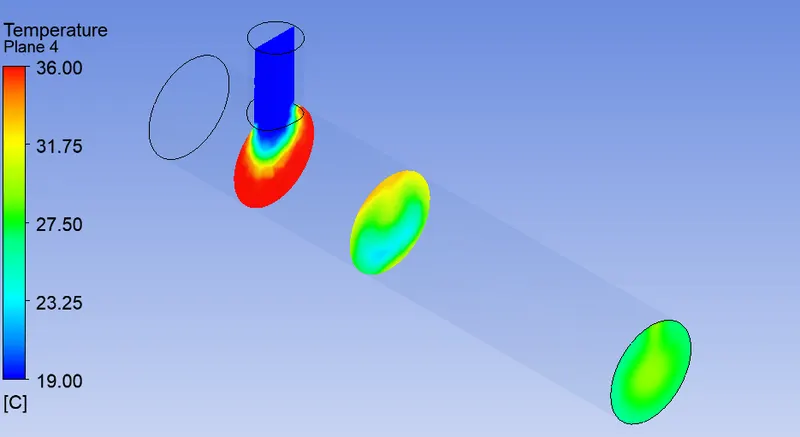
• Isometric view of temperature distribution on planes across the tee at different locations of tee. 

                             

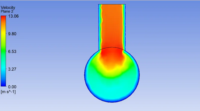
• Velocity distribution on a plane across the tee at the cross section where fluid from two inlets meet.

                            

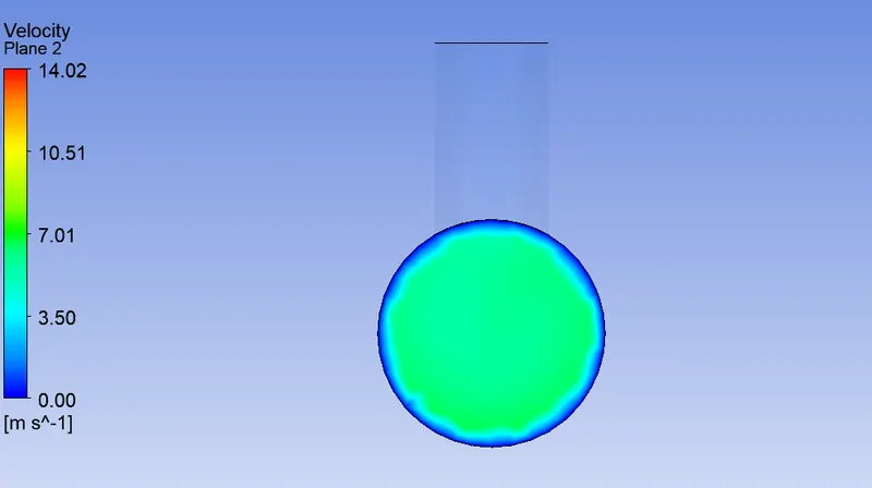
• Velocity distribution on a plane across the tee at the outlet of mixed tee. 

                            

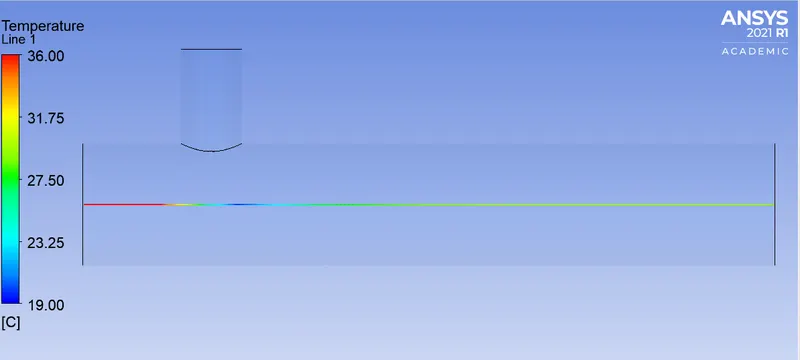
• Temperature distribution on a line plot along the length of tee.

                            

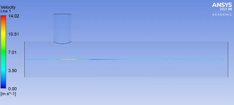
• Velocity distribution on a line plot along the length of tee.         

                           

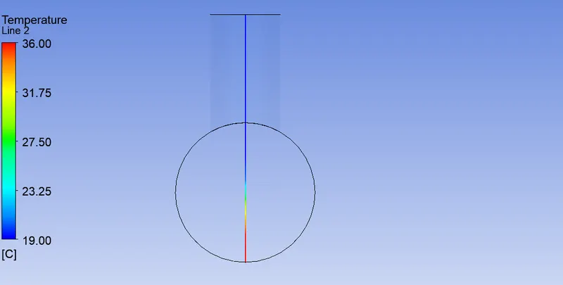
• Temperature distribution on a line plot across the length of tee at the cross section where fluid from two inlets meet.

                        

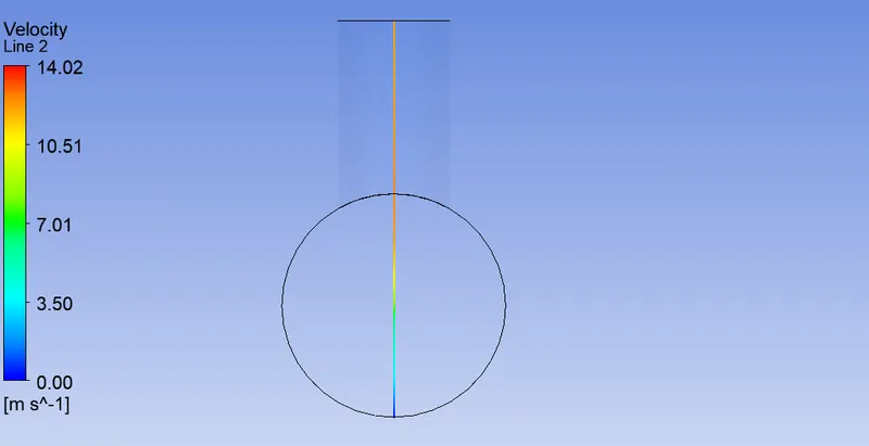
• Velocity distribution on a line plot across the length of tee at the cross section where fluid from two inlets meet.

                        

• Temperature distribution on a line plot across the length of tee at the outlet.

                        

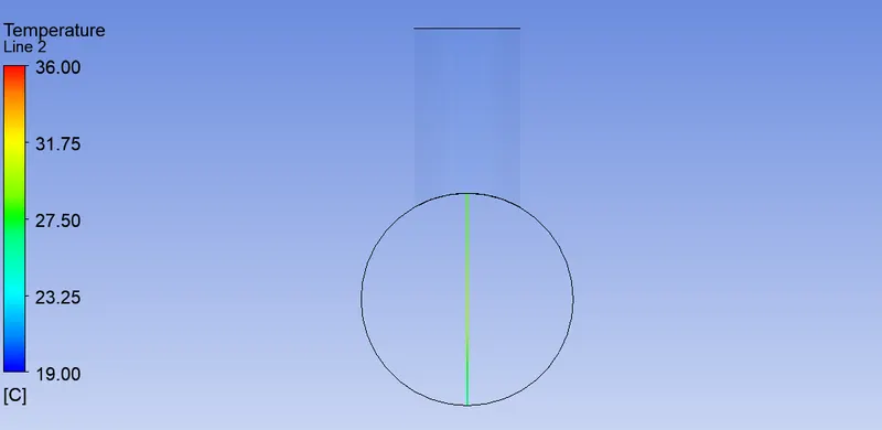
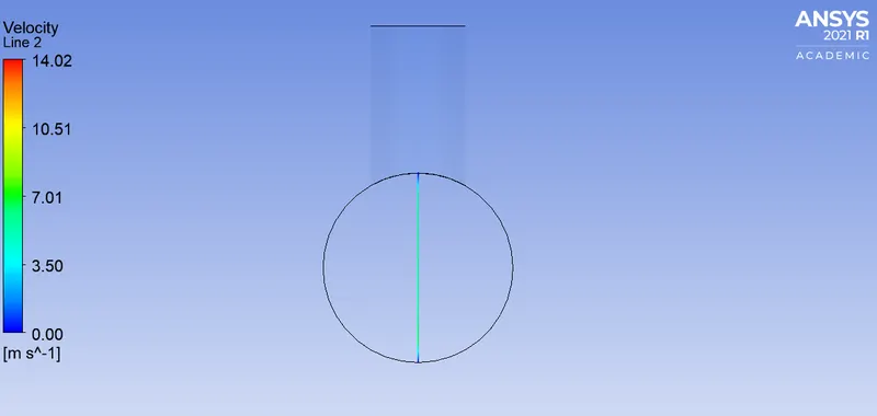
• Velocity distribution on a line plot across the length of tee at the outlet.

                      

Case 2  :   a) Long mixing tee with a hot inlet velocity of 3m/s and Momentum ratio of 2 :

• We will follow the same steps starting from extracting the volume then meshing and then to the solution setup procedure.
• To set up our problem we open Fluent and setup inital conditions , boundary conditions material etc.,
• We first start with checking the mesh quality using perform mesh check under domain.If no error is seen in console window then we can proceed further.
• Then we move move to setting up physics where we select the solver ,viscous model ,initial and boundary conditions etc.,
• We use a steady state pressure based solver to solver our model.

Physics :

General :

                     Solver type      :      pressure based

                         time            :      steady state

      velocity formulation         :       absolute

• Then we select the k - epsilon realizable model which is upgraded version of k -epsilon model with standard wall functions.Here we have to selecct the energy equation as we are solving for the temperature.

models  :

                      viscous model  :        k-epsilon

                        type             :       realizable 

            Near wall treatment   :       standard wall functions

• Here we use air as our working fluid.

Material  :

                       name           :       air

Zones :

                  Cell zone :  you will see our volume zone which is basically our internal volume basically mesh, and it is of type fluid.You can also change material name here if required.

  Boundary conditions :We will basically give our boundary conditions here such as inlet velocity and temperature and outlet conditions.

                       given our  inlet x velocity =3 m/sec and momentum ratio = 2 then ,  

                       Momentum ratio = velocity at cold inlet(y) / velocity at hot inlet(x),

                       => velocity at cold inlet(y) = 3*2 = 6m/sec 

   inlet -x :  

                      velocity      :      3 m/sec

               Temperature     :     36 °C

   inlet -y :  

                      velocity     :    6 m/sec

               Temperature    :    19 °C

 outlet  :

      pressure outlet : gauge pressure = 0 pa

• Now we are almost ready to run the simulation ,but as the solution is being solved we want to moniter some physical quantity during the run time ,here we need to moniter the outlet temperature.

        steps :  solution -> under definitions -> select new -> select the surface report ->area weighted average-> and select the parameter you want to moniter-> check report file and report plot ->then okay.

• Here we will moniter temperature and standard deviation of temperature at the outlet ,which is used to know the mixing effectiveness its low value is equal to very good mixing.

          steps :  solution -> under definitions -> select new -> select the surface report ->standard deviation->temperature at outlet -> check report file and report plot ->then okay.

• Finally after the setting up of initial conditions and boundary conditions the next thing to do is initialization.

Initialization :

When performing CFD analysis  ,as we are solving for pressure and velocity and temperature and other variables we need to provide starting values for all these variable at all cells at t=0.

        steps : solve -> initialization -> Hybrid -> initialize (t=0) 

• The next thing to do is run by clicking calculate.We run for 333 iterations 
• Then we can see that in the residual plot we see residuals dropping and reach a steady state after 180 iterations.

•                          

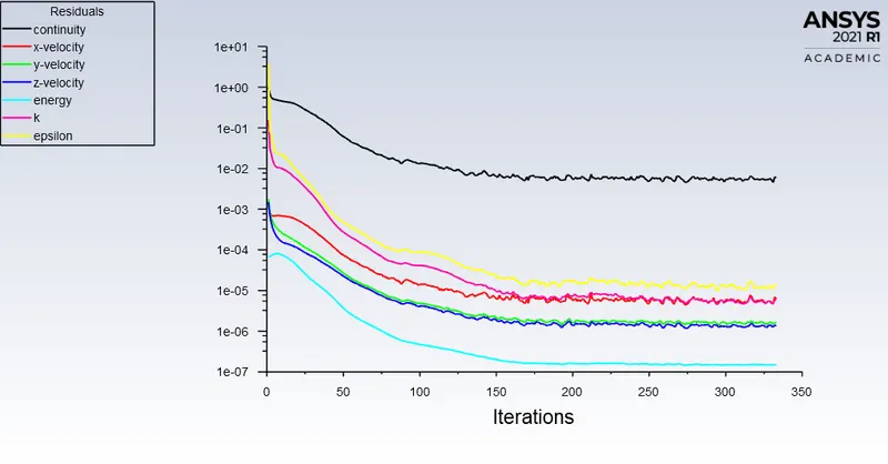
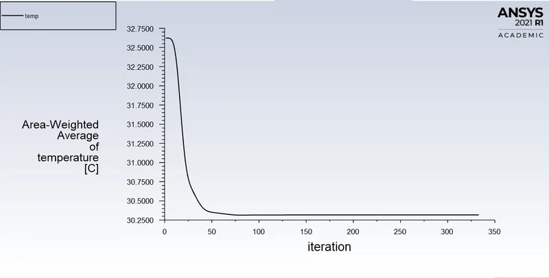
• In the report of average outlet temperature you will see the temperature is 30.316 °C which almost steady after 75 iterations   

•                          

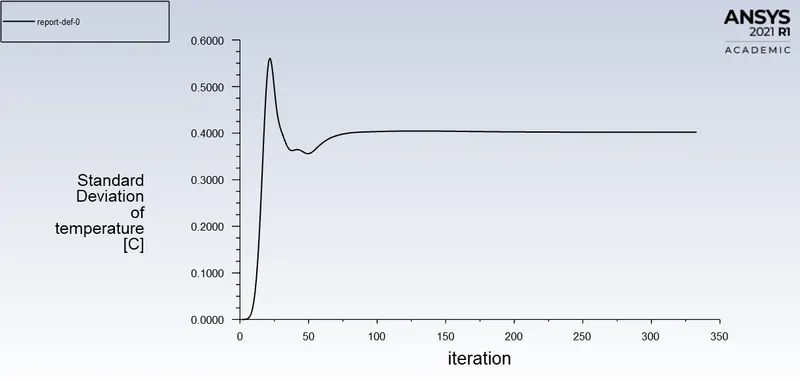
• In the report of standard deviation of  temperature at the outlet you will see it is 1.478 which almost steady after 120 iterations.

•                         

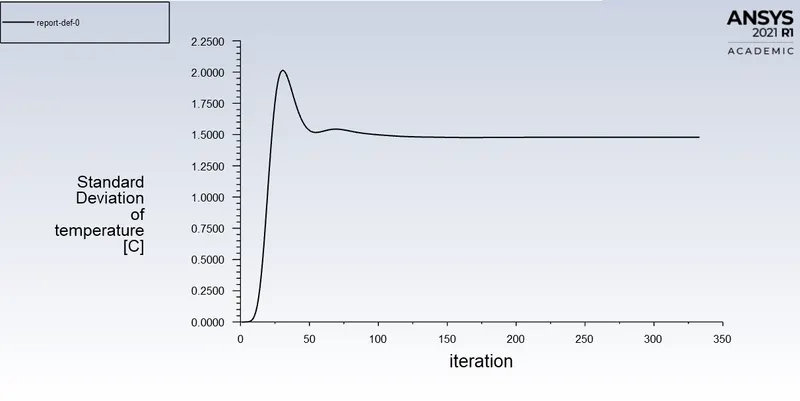
• Now, lets post process the results which we obtained by the above simulation.
• Contour of Temperature distribution on a plane along the length of tee.

•                         

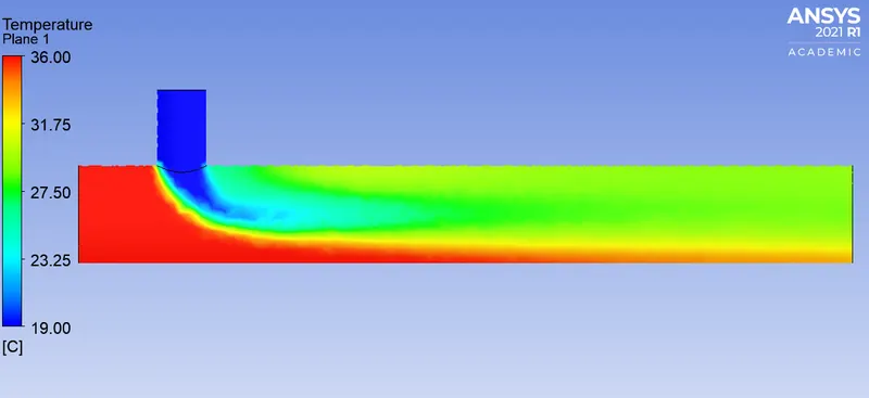
• Contour of velocity distribution on a plane along the length of tee.

                               

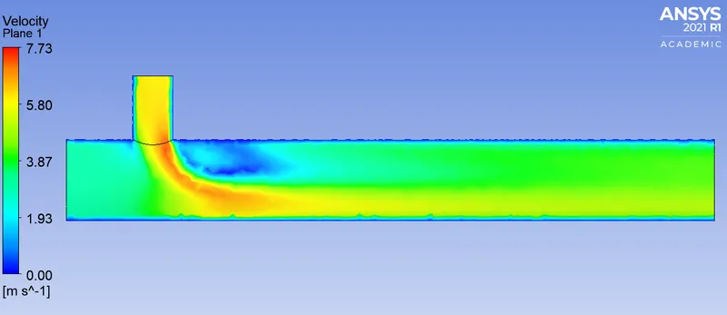
• Contour of pressure distribution on a plane along the length of tee.

                               

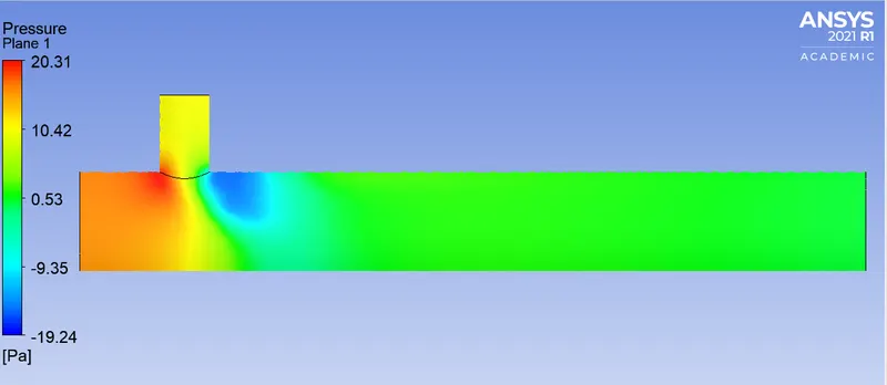
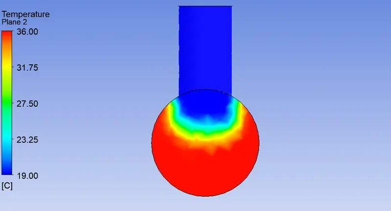
• Temperature distribution on a plane across the tee at the cross section where fluid from two inlets meet.

                               

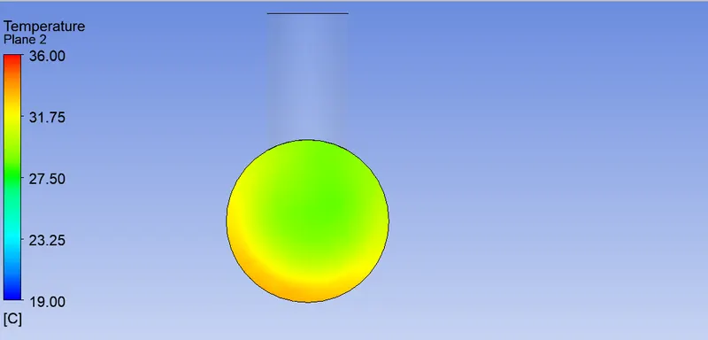
• Temperature distribution on a plane across the tee at the outlet of mixed tee. 

                               

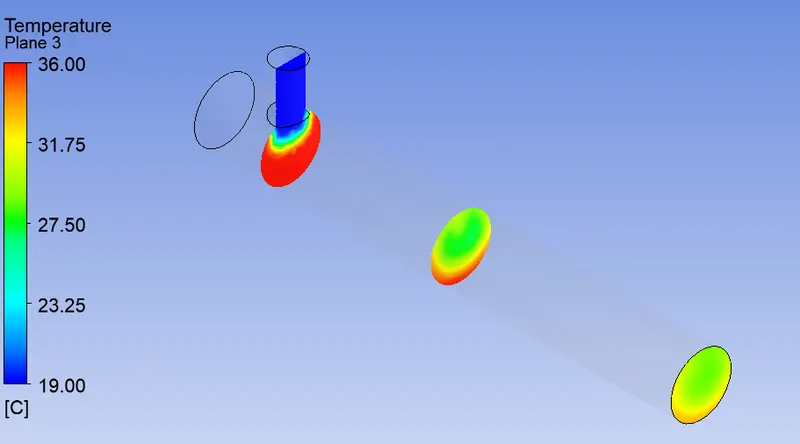
• Isometric view of temperature distribution on planes across the tee at different locations of tee. 

                                

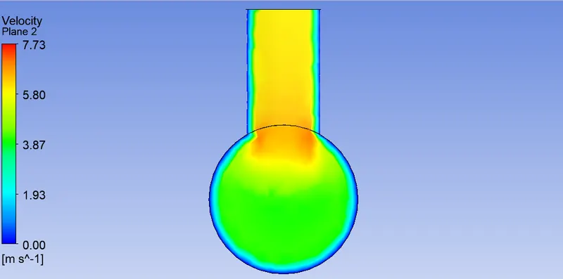
• Velocity distribution on a plane across the tee at the cross section where fluid from two inlets meet.

•                        

• Velocity distribution on a plane across the tee at the outlet of mixed tee. 

•                        

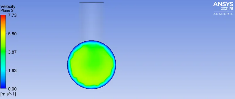
• Temperature distribution on a line plot along the length of tee.

•                       

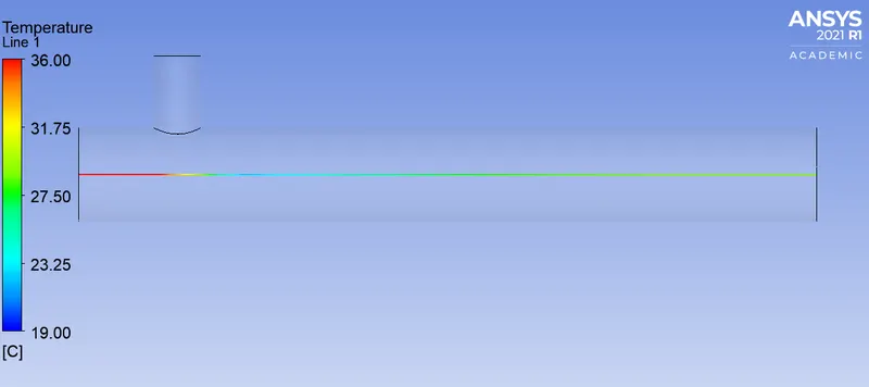
• Velocity distribution on a line plot along the length of tee.         

•                      

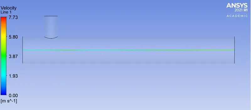
• Temperature distribution on a line plot across the length of tee at the cross section where fluid from two inlets meet.

•                    

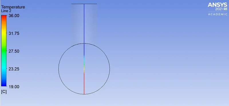
• Velocity distribution on a line plot across the length of tee at the cross section where fluid from two inlets meet.

•                     

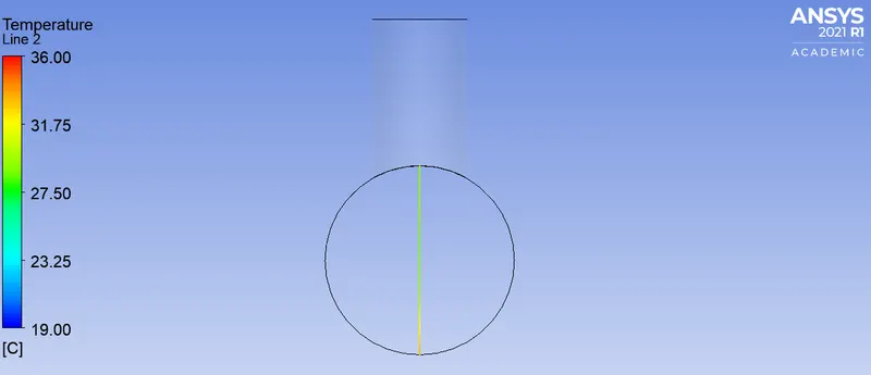
• Temperature distribution on a line plot across the length of tee at the outlet.

•                   

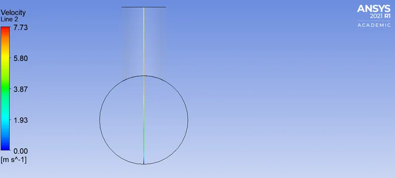
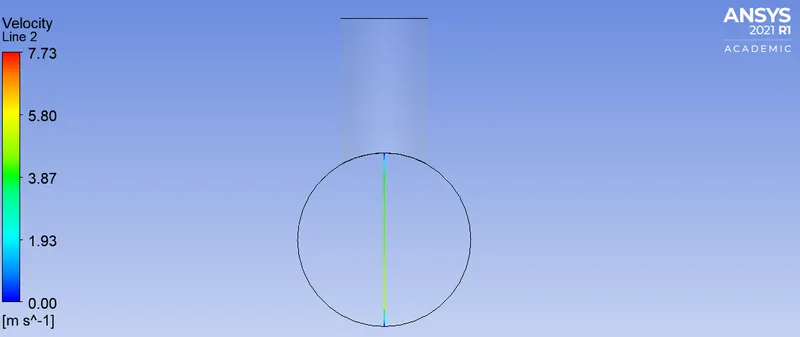
• Velocity distribution on a line plot across the length of tee at the outlet.

                          

b) Long mixing tee with a hot inlet velocity of 3m/s and Momentum ratio of 4 :

• We will follow the same process but we will have a different inlet velocity in y-direction as our momentum ratio changed.
• First we start with setting up physics where we select the solver ,viscous model ,initial and boundary conditions etc.,We use a steady state pressure based solver to solver our model.

Physics :

General :

                     Solver type      :      pressure based

                         time            :      steady state

      velocity formulation         :       absolute

• Then we select the k - epsilon realizable model which is upgraded version of k -epsilon model with standard wall functions.Here we have to selecct the energy equation as we are solving for the temperature.

models  :

                      viscous model  :        k-epsilon

                        type             :       realizable 

            Near wall treatment   :       standard wall functions

• Here we use air as our working fluid.

Material  :

                       name           :       air

Zones :

                  Cell zone :  you will see our volume zone which is basically our internal volume basically mesh, and it is of type fluid.

  Boundary conditions :We will basically give our boundary conditions here such as inlet velocity and temperature and outlet conditions.

                       given our  inlet x velocity =3 m/sec and momentum ratio = 4 then ,  

                       Momentum ratio = velocity at cold inlet(y) / velocity at hot inlet(x),

                      =>  velocity at cold inlet(y) = 3*4 = 12m/sec 

   inlet -x :  

                      velocity      :      3 m/sec

               Temperature     :     36 °C

   inlet -y :  

                      velocity     :    12 m/sec

               Temperature    :    19 °C

 outlet  :

      pressure outlet : gauge pressure = 0 pa

• Now we are almost ready to run the simulation ,but as the solution is being solved we want to moniter some physical quantity during the run time ,here we need to moniter the outlet temperature.

        steps :  solution -> under definitions -> select new -> select the surface report ->area weighted average-> and select the parameter you want to moniter-> check report file and report plot ->then okay.

• Here we will moniter temperature and standard deviation of temperature at the outlet ,which is used to know the mixing effectiveness its low value is equal to very good mixing.

          steps :  solution -> under definitions -> select new -> select the surface report ->standard deviation->temperature at outlet -> check report file and report plot ->then okay.

• Finally after the setting up of initial conditions and boundary conditions the next thing to do is initialization.

Initialization :

When performing CFD analysis  ,as we are solving for pressure and velocity and temperature and other variables we need to providde starting values for all these variable at all cells at t=0.

        steps : solve -> initialization -> Hybrid -> initialize (t=0) 

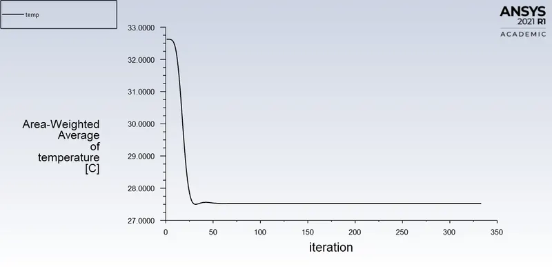
• The next thing to do is run by clicking calculate.We run for 333 iterations 
• Then we can see that in the residual plot we see residuals dropping and reach a steady state after 175 iterations.

                         

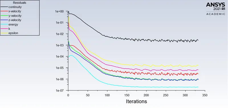
• In the report of average outlet temperature you will see the temperature is 27.527 °C which almost steady after 55 iterations   

                          

• In the report of standard deviation of  temperature at the outlet you will see it is 0.402 which almost steady after 85 iterations.

                          

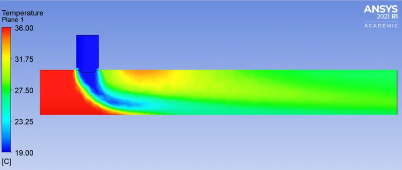
• Now, lets post process the results which we obtained by the above simulation.
  • Contour of Temperature distribution on a plane along the length of tee.

                          

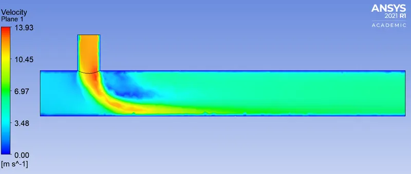
• Contour of velocity distribution on a plane along the length of tee.

                           

• Contour of pressure distribution on a plane along the length of tee.

                           

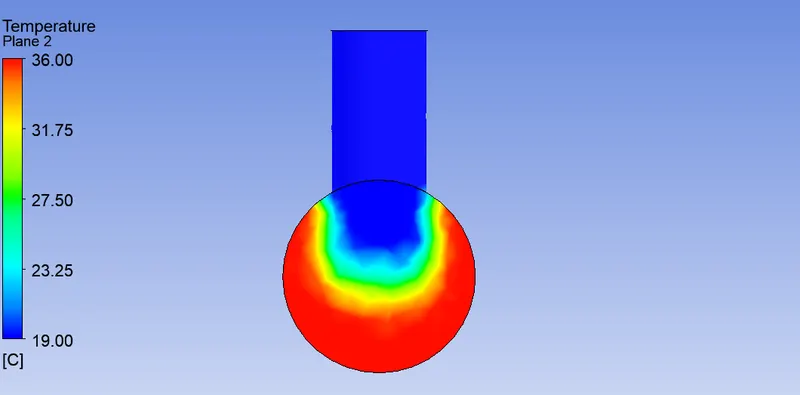
• Temperature distribution on a plane across the tee at the cross section where fluid from two inlets meet.                       

                           

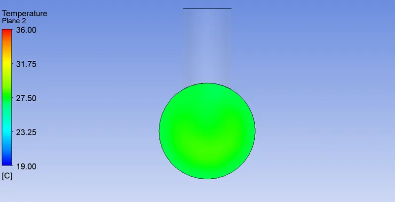
• Temperature distribution on a plane across the tee at the outlet of mixed tee. 

                           

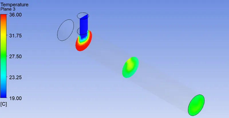
• Isometric view of temperature distribution on planes across the tee at different locations of tee. 

                            

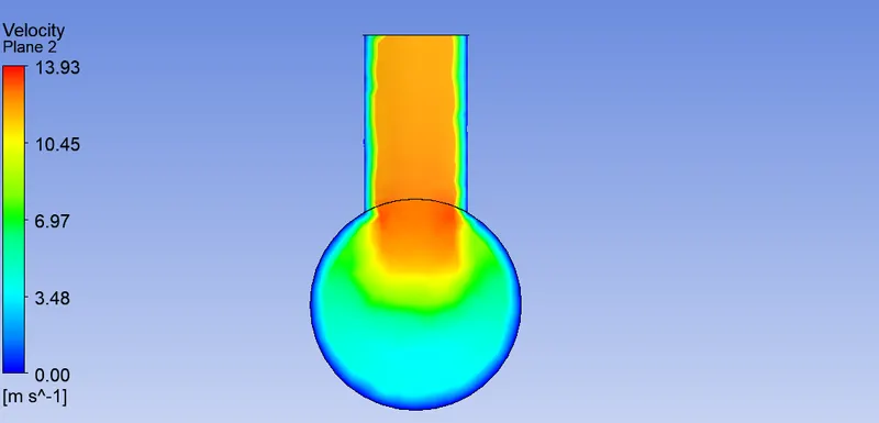
• Velocity distribution on a plane across the tee at the cross section where fluid from two inlets meet.

                           

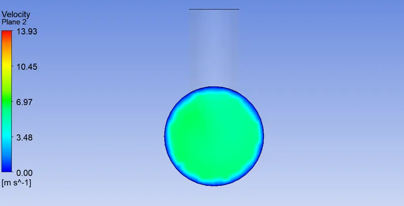
• Velocity distribution on a plane across the tee at the outlet of mixed tee. 

                           

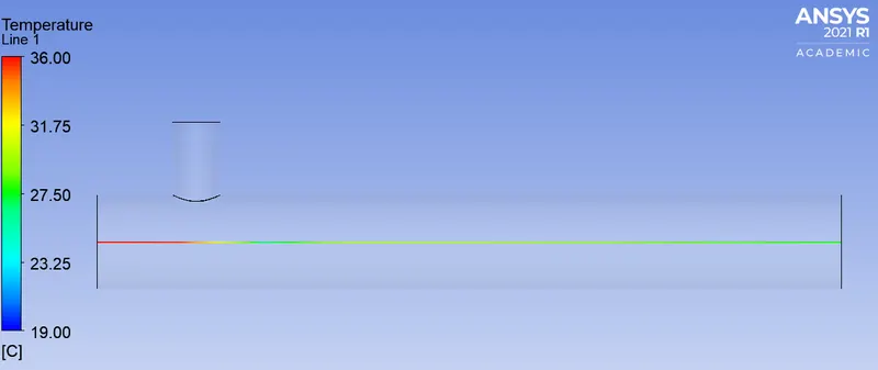
• Temperature distribution on a line plot along the length of tee.

                          

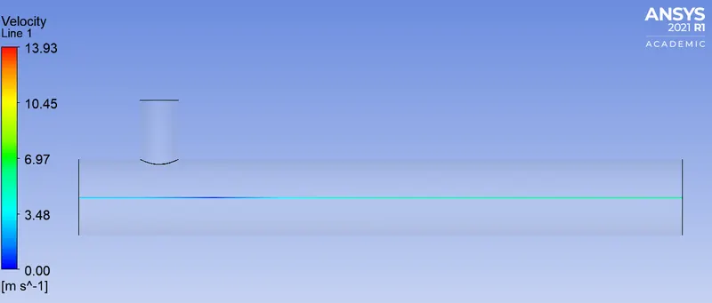
• Velocity distribution on a line plot along the length of tee.         

                         

• Temperature distribution on a line plot across the length of tee at the cross section where fluid from two inlets meet.

                       

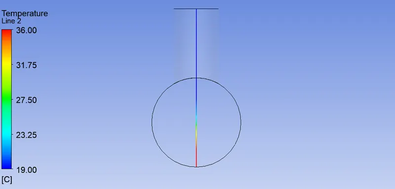
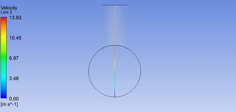
• Velocity distribution on a line plot across the length of tee at the cross section where fluid from two inlets meet.

                      

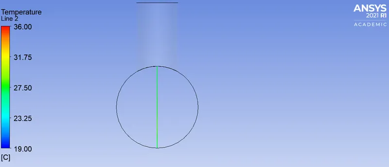
• Temperature distribution on a line plot across the length of tee at the outlet.

                     

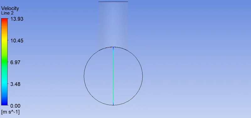
• Velocity distribution on a line plot across the length of tee at the outlet.

                    

Mesh independent study :

• To do mesh independent study first we have to start by selecting a case and then we have to simulate it with different mesh sizes.
• We will consider our first case i.e., short mixing tee with a hot inlet velocity of 3 m/s and Momentum ratio of 2 .
• Now let us simulate the above case with three different mesh sizes i.e.,0.003m ,0.002m ,0.0015m,0.0011m and then tabulate the results.
• The first size we have already simulated above now let us simulate for the other three grid sizes then tabulate and discuss the results.   

              

• From the above table we can observe that with the decrease in grid size results in a value which is getting very close to the analytical solution.
• We can also observe that almost all the values are equal but there is a difference in the range of 1e-2.
• The thing is with the decrease in the grid size there will be increase in computational effort.
• So the results which we got by taking the grid size as 3mm are very much satisfactory and very close to the analytical solution. 
• So we can conclude that our result is grid dependent.

Effect of length and momentum ratio on results :

• To conclude let us tabulate all the results of four cases to discuss the effect of length and momentum ratio on results.

                

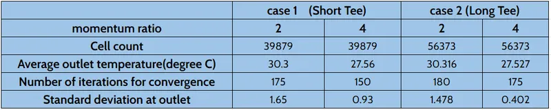
• From the above table we can conclude that when we increase the momentum ratio we can see that the mixing is efficient which we can conclude by seeing the standard deviation,Which leads to a less outlet temperature.
• When we increase the length of the tee we can see that the mixing is efficient, and for the same momentum ratio the effective temperature at the outlet is quite close to the analytical solution when we increase the length.

Animation : 

Animation of temperature distribution of mixed tee : 

                                         

Temperature distribution animation on a plane (Mixed Tee) :