Week 7 - Simulating Fluid Sloshing effect inside a Gear-box

Objective :

In this challenge,

• We will discuss what is Dynamic meshing and some other examples where dynamic meshing can be used.
• And then we discuss about the fluid Sloshing effect and discuss whether the sloshing effect is good or bad.
• Then we discuss what is the use of UDF.
• Then we come to main part i.e., we will perform four simulations in the Gearbox and then we will compare the results among all the four cases.The four cases are,

1. 20% Immersion, Fluid - Engine oil.
2. 30% Immersion, Fluid- Engine oil.
3. 20% Immersion,Fluid-n-heptane (c7h16).
4. 30% Immersion,Fluid-n-heptane (c7h16).

• Finally we will discuss the common errors that will occur in the simulation. A] 'Dynamic mesh failed' error. B] 'Negative cell volume detected' error.

Introduction :

• This type of analysis is commonly used in the industries to checkout ,if a given gearbox setup with a particular lubricant is adequately reaching all the teeth and if adequate performance is achieved by the gear.Let us start with some theory about dynamic meshing fluid sloshing and UDF's.

Dynamic meshing :

• The dynamic mesh model allows you to move the boundaries of a cell zone relative to other boundaries of the zone, and to adjust the mesh accordingly. The boundaries can move rigidly with respect to each other (that is, linear or rotational motion), and/or deform.
• The motion of the boundaries can be rigid, such as pistons moving inside an engine cylinder or a flap deflecting on an aircraft wing, or deforming, such as the elastic wall of a balloon during inflation or a flexible artery wall responding to the pressure pulse from the heart. In either case, the nodes that define the cells in the domain must be updated as a function of time, and hence the dynamic mesh solutions are inherently unsteady.
• An important special case of dynamic mesh motion is called the sliding mesh in which all of the boundaries and the cells of a given mesh zone move together in a rigid-body motion. In this situation, the nodes of the mesh move in space (relative to the fixed, global coordinates), but the cells defined by the nodes do not deform. Furthermore, mesh zones moving adjacent to one another can be linked across one or more non-conformal interfaces. As long as the interfaces stay in contact with one another (that is, “slide” along a common overlap boundary at the interface), the non-conformal interfaces can be dynamically updated as the meshes move, and fluid can pass from one zone to the other.
• The dynamic mesh model in ANSYS Fluent can be used to model flows where the shape of the domain is changing with time due to motion on the domain boundaries. The dynamic mesh model can be applied to single or multiphase flows (and multi-species flows). The update of the volume mesh is handled automatically by ANSYS Fluent at each time step based on the new positions of the boundaries. To use the dynamic mesh model, you need to provide a starting volume mesh and the description of the motion of any moving zones in the model. ANSYS Fluent allows you to describe the motion using either boundary profiles, user-defined functions (UDFs), or the six degrees of freedom solver.
• ANSYS Fluent expects the description of the motion to be specified on either face or cell zones. If the model contains moving and non-moving regions, you need to identify these regions by grouping them into their respective face or cell zones in the starting volume mesh that you generate. Furthermore, regions that are deforming due to motion on their adjacent regions must also be grouped into separate zones in the starting volume mesh. The boundary between the various regions need not be conformal. You can use the non-conformal or sliding interface capability in ANSYS Fluent to connect the various zones in the final model.
• Three groups of mesh motion methods are available in ANSYS Fluent to update the volume mesh in the deforming regions subject to the motion-defined at the boundaries.

1. Smoothing Methods.
2. Dynamic Layering.
3. Remeshing Methods.

1. Smoothing Methods:

• When smoothing is used to adjust the mesh of a zone with a moving and/or deforming boundary, the interior nodes of the mesh move, but the number of nodes and their connectivity does not change. In this way, the interior nodes “absorb” the movement of the boundary.

2. Dynamic layering:

You can use the dynamic layering method to split or merge cells adjacent to any moving boundary provided if the following conditions are met:

• All cells adjacent to the moving face zone are either wedges or hexahedra (quadrilaterals in 2D) even though the cell zone may contain mixed cell shapes.
• The cell layers must be completely bounded by one-sided face zones, except when sliding interfaces are used.

3. Remeshing Methods:

• When the boundary displacement is large compared to the local cell sizes, the cell quality can deteriorate or the cells can become degenerate if only mesh smoothing is used. This will invalidate the mesh (for example, result in negative cell volumes) and consequently, will lead to convergence problems when the solution is updated to the next time step.
• To circumvent this problem, ANSYS Fluent agglomerates cells that violate the skewness or size criteria and locally remeshes the agglomerated cells or faces. If the new cells or faces satisfy the skewness criterion, the mesh is locally updated with the new cells (with the solution interpolated from the old cells). Otherwise, the new cells are discarded and the old cells are retained.
• ANSYS Fluent includes several remeshing methods that include local cell remeshing, zone remeshing, local face remeshing (for 3D flows only), face region remeshing, and 2.5D surface remeshing (for 3D flows only).

Fluid Sloshing effect :

• In fluid dynamics, slosh refers to the movement of liquid inside another object (which is, typically, also undergoing motion).
• Strictly speaking, the liquid must have a free surface to constitute a slosh dynamics problem,where the dynamics of the liquid can interact with the container to alter the system dynamics significantly. Important examples include propellant slosh in spacecraft tanks and rockets (especially upper stages), and the free surface effect (cargo slosh) in ships and trucks transporting liquids (for example oil and gasoline). However, it has become common to refer to liquid motion in a completely filled tank, i.e. without a free surface, as "fuel slosh".
• Such motion is characterized by "inertial waves" and can be an important effect in spinning spacecraft dynamics. Extensive mathematical and empirical relationships have been derived to describe liquid slosh. These types of analyses are typically undertaken using computational fluid dynamics and finite element methods to solve the fluid-structure interaction problem, especially if the solid container is flexible.
• The fluid sloshing effect can be good or bad depending upon the case. In some cases it is desirable have sloshing effect e.g. sloshing of lubricant in gearbox, mixing tanks. Whereas, in some cases sloshing is having adverse effects e.g. partially filled container on locomotive
• Slosh is an important effect for spacecraft, ships and road tank vehicles.
• Liquid sloshing strongly influences the directional dynamics and safety performance of highway tank vehicles in a highly adverse manner.Hydrodynamic forces and moments arising from liquid cargo oscillations in the tank under steering and/or braking maneuvers reduce the stability limit and controllability of partially-filled tank vehicles.Anti-slosh devices such as baffles are widely used in order to limit the adverse liquid slosh effect on directional performance and stability of the tank vehicles. Since most of the time, tankers are carrying dangerous liquid contents such as ammonia, gasoline and fuel oils, stability of partially-filled liquid cargo vehicles is very important. Optimizations and sloshing reduction techniques in fuel tanks such as elliptical tank, rectangular, modified oval and generic tank shape have been performed in different filling levels using numerical, analytical and analogical analyses. Most of these studies concentrate on effects of baffles on sloshing while the influence of cross-section is completely ignored.
• Sloshing or shifting cargo, water ballast, or other liquid (e.g., from leaks or fire fighting) can cause disastrous capsizing in ships due to free surface effect; this can also affect trucks and aircraft.

UDF and its uses :

• A user-defined function (UDF) is a function provided by the user of a program or environment, in a context where the usual assumption is that functions are built into the program or environment. UDFs are usually written for the requirement of its creator.
• UDF's allow you to customize Ansys Fluent and can significantly enhance its capabilities.
• A user-defined function, or UDF, is a function that you program that can be dynamically loaded with the ANSYS FLUENT solver to enhance the standard features of the code.

• UDF can be used for a number of applications like :

  1. To define dynamic motion of the required parts.
  2. Customize boundary conditions
  3. Material property definitions
  4. Adjust computed values on a once-per-iteration basis
  5. Initialize with a previous solution
  6. Enhance post-processing
  7. Enhance existing ANSYS FLUENT models (such as discrete phase model, multiphase mixture model, discrete ordinates radiation model)

Solution procedure :

• We wil simulate all the four cases with the transient state.We will not simulate the 3D case because of the limitation af academic license.So, we are going to simulate 2D part by using the user defined function(UDF). For solving we follow the below procedure :

1)Geometry setup

2)Meshing

3) Problem setup

4)Solving

5)Post processing

Simulating the flow with the transient solver :

Case -1 :- 20% of immersion with fluid - Engine oil :

1) Geometry setup :

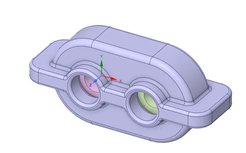
• In fluent module we have to open spaceClaim and then import the 3D geometry.The below image is the 3D view of gear box.

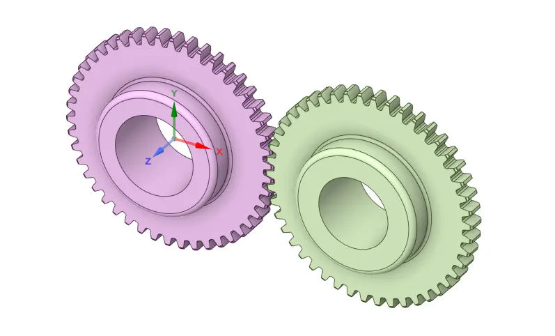
• You can see the left gear and right gear more clearly if you hide the housing.The below image is the 3D view of gears.

• We need to extract the fluid volume first.For that ,

steps : prepare -> volume extract -> select the fluid volume by selecting all the edges of 4 openings -> Then ok.

• Then new object will be added to the tree.Then hide the solid volume and the left is fluid volume which we generated.
• Now we have to split this body into half to extract the 2D geometry right in the middle plane.
• First create planes by selecting plane in design and click on origin ,which creates 2 planes X,Y and Z planes.
• We use the split body command in spaceclaim which is under design to split the geometry it into two parts by selecting the geometry and plane and delete the other part.
• Now we can see the interior sectional view.Now if you select the top part of the remaining geometry you can see the yellow top face part,which is what we want .Inorder to extract that area we need to select that face and copy and open new design and then paste it and save it.
• Now reset the setup and import the 2D saved geometry and open the meshing module.
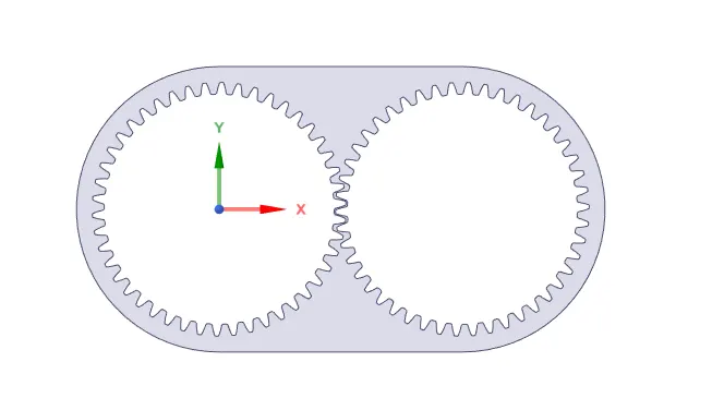
• The below image is the final 2D geometry that we simulate.

2) Meshing :

• For meshing we open Meshing,where we mesh our model so that we can use it to solve our model.
• In general it is always good to name the surfaces before meshing. So let us do that.
• We have to give the name for left and right set of gear teeth,so that while import the UDF you can give left motion to left set of gears and right motion to right set of gears.
• We first select the edges of left gear by using the edge selection so that we can provide name for our entity selection.

steps : select all the edges of left gear by using edge selection properly without missing any edge of gear teeth -> then press N -> name the selection as left_gear.

• In the similar way we name the right_gear.
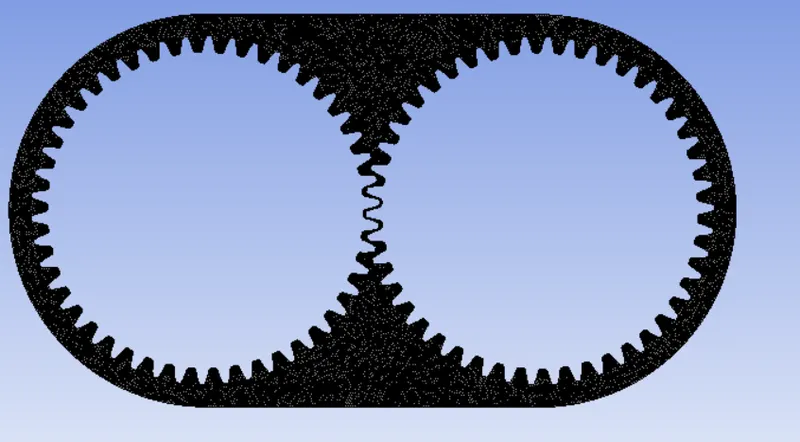
• Then next thing to do is to mesh.We click the mesh option in the side then give element size as 0.8 mm and also select capture curvature and proximity to on and generate mesh.
• The below image is the final view of mesh .

• Now we have to check the quality of the mesh.

steps : mesh ->quality-> mesh metric-> Element quality

• Here our minimum quality is around 15 %,so we can move further for our solution setup.

3) Problem Setup :

• To set up our problem we open Fluent and setup inital conditions , boundary conditions material etc.,
• We first start with checking the mesh quality using perform mesh check under domain.If no error is seen in console window then we can proceed further.
• Then we move move to setting up physics where we select the solver,viscous model etc.
• We use a transient state pressure based solver to solve our model.

Physics :

General :

Solver type : pressure based

time : transient state

velocity formulation : absolute

• We need to enable gravity by giving value for Y as -9.8 m/s^2 as gravity is acting in negative Y-direction.

models :

viscous model : K-epsilon realizable model with enhanced wall treatment.

Material : Fluid -1 : Air

Fluid -2: Engine oil (density - 880 kg/m^3 , Viscosity - 0.121 kg/ms )

In models enable multiphase flow and in that select,

for model : select VOF method

Number of Eulerian phases : 2

Formulation : Implicit

• And in phases option as we selected two phases give names and selcect phase ,
• For primary phase :change name as air and change phase material to air
• For secondary phase :change name as water and change phase material to engine oil .
• Then for doing patching we have to initialize first and then we do Hybrid initialization .
• But,before initialization we have to mark or define a region of cells where the fluid has to be i.e.,20% of immersion to get the 20% of the height we note from the spaceclaim. We also note the centre of gravity location which we use while defining the dynamic mesh.WE mark by using the adapt/mark and create a region a give the values which creates required region.
• In patch for phase select engine oil and for variable you can see volume fraction now .
• Now, patch the value fraction value of 0 to other domain and 1 to the region we have just created which you can find in the registers to patch.
• Now we are almost ready to run the simulation but as to verify the patching,we create contour for volume fraction of water .
• Now we can verify the patching by creating contour of volume fraction of engine oil.
• For contour -> go to solutions tab -> graphics -> contour -> in contour of : select phases and under that select volume fraction and for phase select engine oil -> select whole domain and press save /display.
• Then you can see the initial values for volume fraction of engine oil on whole domain,where you can see in the bottom it is set to 1 and for the top region it is set to 0.So we can conclude that our initialization is correct.
• Then we have to setup the dynamic mesh.
• For that we have to load the UDF ,select, under user defined -> select function -> and that select compiled -> then add and use built in compiler to build the UDF and then load it.
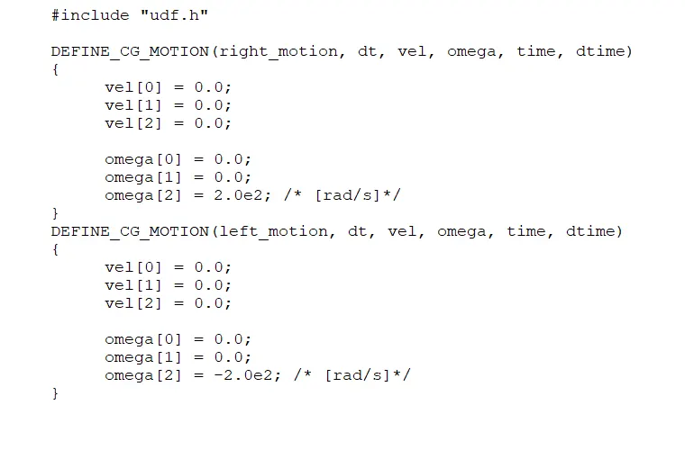
• The below code is the UDF we use here.

• Now in mesh module select dynamic mesh and under that select smoothing, layering and remeshing.Then we have to create dynamic mesh zones.
• Select create under dynamic mesh zones and we have to create,
• For left gear -> select for type - rigid body -> for motion UDF/profile - select left motion -> and for centre of gravity - give value as (0,0,0) (which is centre of gravity we noted) -> Then click on create.
• In the same way create right motion by giving ,for motion UDF/profile - we select right motion and for centre of gravity we give value as (0.115,0)m.
• Then you will see two zones created in dynamic zones -left gear and right gear.
• You will see the motion of gears by selecting select display zone motion and set time control and preview.You will see gears rotating .So we can conclude that the UDF has setup successfully.
• Then initialize and patch again and we also want to create animation so that we can see how the solution or volume fraction of water is is varying when problem is being solved.
• For that,

steps : Activities -> solution animation -> select volume fraction contour,which we have created -> preview -> set the required view and use active -> and name it as volume fraction of water animation.

• Then in solution method for Pressure velocity coupling SIMPLE scheme is used. For the momentum second order upwind scheme is used and for pressure, PRESTO is selected. For the transient formulation first order implicit scheme is choosen for better results and for stability and convergence of the residuals.

4) Solving :

• Then we are ready to solve .We run the simulation by giving time step size as 1e-4 and no. of time steps = 1000.
• Here we give angular velocity as 200 rad/sec in the UDF . It means , omega =2*pi*N/60 . => N = 6000/pi = 1909.8593 rpm =31.8309 rotations per second.
• So, for every rotation it is taking 1/31.8309 sec = 0.031416 sec.
• Here we ran for 1000 time steps with time step size = 0.0001. so,total time = 0.1 sec, which means we ran for more than 3 rotations, which is enough for our analysis.
• Then let us post process the results.

5)Post processing :

Residuals plot :

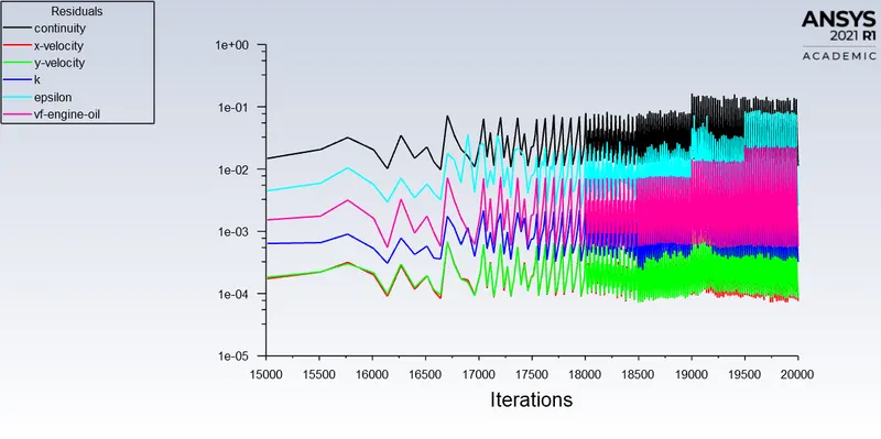
• You can observe from the below plot the residuals has converged.

Animation :

• Animation of fluid sloshing effect inside a gear-box ,with 20% Immersion of gears with fluid - Engine oil.

• So , let us simulate for other three cases and compare the results all at a time.

Case -2 :- 30% of immersion with fluid - Engine oil :

• Everything is same as previous case from the point of geometry and mesh.
• Comming to set up the only change here is the immersion is 30%.So we give different values for coordinates for marking ,here we give coordinates of values 30% of height from base.The fluid is also same for this case.Remaining everything is same as previous case.
• Then we run for 1000 time steps with time step size = 0.0001. and the total run time = 0.1s.
• So let us directly run the simulation and then post process the results.

Post processing :

Residuals plot :

• You can observe from the below plot the residuals has converged.

Animation :

• Animation of fluid sloshing effect inside a gear-box ,with 30% Immersion of gears with fluid - Engine oil.

Case -3 :- 20% of immersion, fluid - n-heptane (c7h16) :

• Everything is same as previous two cases from the point of geometry and mesh.
• Comming to set up the only change is here the immersion is 20%.So we give different values for coordinates for marking , here we give coordinates of values 20% of height from base.Here the fluid is n-heptane (c7h16) for this case.Remaining everything is same as previous cases.
• Then we run for 1000 time steps with time step size = 0.0001. and the total run time = 0.1s.
• So let us directly run the simulation and then post process the results.

Post processing :

Residuals plot :

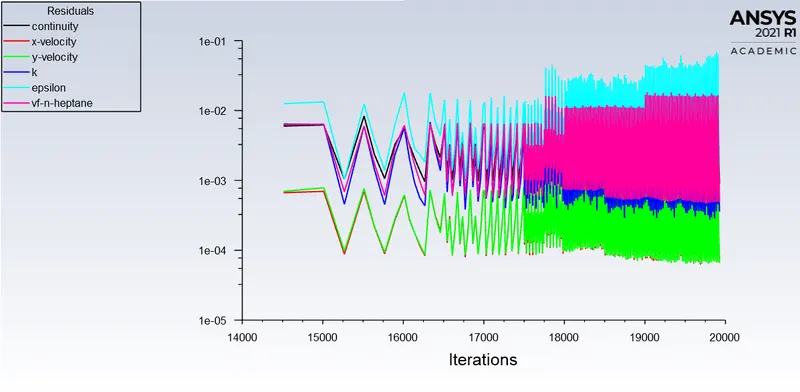
• You can observe from the below plot the residuals has converged.

Animation :

• Animation of fluid sloshing effect inside a gear-box , with 20% Immersion of gears with fluid - n-heptane (c7h16).

Case -4 :- 30% of immersion, fluid - n-heptane (c7h16) :

• Everything is same as previous three cases from the point of geometry and mesh.
• Comming to set up the only change is here the immersion is 30%.So we give different values for coordinates for marking ,here we give coordinates of values 30% of height from base.Here the fluid is n-heptane (c7h16) for this case.Remaining everything is same as previous cases.
• Then we run for 1000 time steps with time step size = 0.0001. and the total run time = 0.1s.
• So let us directly run the simulation and then post process the results.

Post processing :

Residuals plot :

• You can observe from the below plot the residuals has converged.

Animation :

• Animation of fluid sloshing effect inside a gear-box , with 30% Immersion of gears with fluid - n-heptane (c7h16).

Conclusions :

• Here let us conclude by comparing the results between all the cases and discuss the common errors that will occur in the simulation. A] 'Dynamic mesh failed' error. B] 'Negative cell volume detected' error.
• If you see all the animations you will observe that the fluid from the bottom is being carried away by the gear teeth and it meets at the top ,and at the point where the two gear meets the fluid flow upwards and this fluid meeting at the top or comming from the point of contact and the fluid which falls flowing back downwards through the sides of the gear box.You will observe that all of the gears are well lubricated by the fluid and fluid is adequately reaching all the teeth.
• But lubrication is more better when the immersion is more i.e., 30% because there will be some extra fluid to lubricate as when you will see the case 1 and 3 there will some less fluid so all the fluid has been used for the first rotation for the second rotation the sump is almost empty, so it takes time for the top fluid to comeback downwards to the sump but where as when the immersion is 30% as in cases 2 and 4 there is some extra fluid in the sump even after the first rotation which is used to lubricate for the second rotation if some fluid come out at the interface and meet at the top.So the lubrication is more better when the immersion is more.
• When you compare between the fluid used i.e., between case 1,2 and 3,4 ,as engine oil has more viscosity than n-heptane, it sticks very well to the gears and the gear is lubricated better which you can observe by seeing the animations.So of all the cases , in case 2 the gears are very well lubricated i.e., 30% of immersion with fluid engine oil.

common errors that will occur in the simulation :

Dynamic mesh failed error :

• This error arises when there is a failure in updating the dynamic mesh.It may be due to many reasons like negative cell volume etc. .

Negative cell volume detected' error :

• Negative cell volumes are in dynamic simulations usually produced, if the mesh is getting too much compressed/deformed or skewed, so that the mesh quality deteriorates even to a point, where cells turn into negative cell volume as the mesh moves to far at a give time step it leads to negative cells. The negative cell volume error is shown when the mesh has been updated in a way to cause a negative cell volume (non-physical). Possible factors for causing this error include: (1) overlapping nodes; and (2) significant mesh motion (relative to cell size) per step.These factors are related.
• This occurs as fluent do not have enough time to remesh.A more frequent remeshing step might be an applicable solution, before the mesh quality is becoming that bad.Try to reduce the time step to avoid major mesh displacements. Another solution can be to increase the mesh stiffness close to any solid walls in the simulation in order to prevent the strong deformation of boundary layers or near-wall mesh cells .