Week 4 - CHT Analysis on Exhaust port

AIM:

To perform the conjugate heat transfer analysis on the exhaust port model.

OBJECTIVES:

• Calculate the wall(surface) heat transfer coefficient on the internal solid surface & show the velocity & temperature contours in appropriate areas.
• Maintain the y+ value according to the turbulence model and justify the results.
• verify if the Heat transfer coefficient predictions from the simulations are right and factors the accuracy of the prediction depends.

THEORY OF CONJUGATE HEAT TRANSFER

Conjugate heat transfer corresponds with the combination of heat transfer in solids and heat transfer in fluids. In solids, conduction often dominates whereas, in fluids, convection usually dominates. Conjugate heat transfer is observed in many situations. The exchange of thermal energy between the two physical bodies is called a study of Heat Transfer, the rate of transferred heat is directly proportional to the temperature difference between the bodies.

modes of heat transfer

1. Conduction: diffusion of heat due to temperature gradients. A measure of the amount of conduction for a given gradient is heat conductivity.
2. Convection: when heat is carried away by moving fluid. The flow can either be caused by external influences, forced convection; or by buoyancy forces, natural convection.

FOURIER LAW OF HEAT CONDUCTION

It states that in-plane layer, the heat conduction rate is proportional to the temperature difference and the heat transfer area across the layer, but inversely proportional to the thickness of the layer(Note: negative sign denotes the heat transfer in the direction of decreasing temperature).

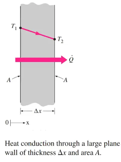
`Qcond=-kA(dt/dx)`

whereas Qcond= conductive heat transfer

k= Thermal conductivity

A= normal surface area

`(dt/dx)`= temperature gradient

NEWTON LAW OF COOLING

It states that convective heat transfer is proportional to the difference in the temperature between an object and its surroundings.

`Qconv=hAtriangleT`

whereas Qconv= convective heat transfer

h= convective heat transfer coefficient

A= normal surface area

`triangleT`= Temperature difference

The convective heat transfer coefficient is not the property of the fluid. It is an experimentally determined parameter whose value depends on all the variables influencing convection such as the surface geometry, nature of the fluid motion, property of the fluid, and bulk fluid velocity.

NUMERICAL ANALYSIS

For this simulation, we are using the K-omega model

Diameter of the pipe=0.166m

velocity=5m/s

Y+=10

first layer thickness=0.5mm

the density of air=1.225 kg/m3

`mu`=1.789*10^-5

Since it is an internal flow and a turbulent model is used, hence the nusselt number formula

`Nu=0.023*Re^0.8*Pr^0.3`

From the heat and mass transfer data book values of thermal conductivity and Prandtl number are taken based on air temperature at 700K

thermal conductivity(k)=0.028 W/mK

Prandtl number(Pr)=0.71

`Re=(rho*v*D)/mu`

we get Re=56833

`Nu=0.023*(56833)^0.8*(0.71)^0.3`

Nu=130

we know that the nusselt number can also be represented as

`Nu=(h*D)/k`

hence rearranged we get

`h=(Nu*k)/D`

`h=(130*0.028)/0.166`

h=21.9277

Hence the obtained heat transfer coefficient from the numerical calculation is 21.9277

EXHAUST PORT:

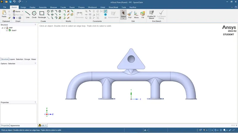
The exhaust port consists of 4 inlet ports and 1 outlet port(diameter of the both ports is 0.166m). We are going to consider the air as the working medium also the boundary condition we are going to take is the velocity (v=5m/s) and temperature (T=700k). Here there are going to be two convective heat transfers happening one is the air entering the pipe and the other air to the internal wall of the pipe we need a convective heat transfer coefficient. Also from the pipe, if it's not an adiabatic wall again there is heat transfer from the pipe to the air. Basically, there will be heat transfer to the air hence we have to consider the domain around the exhaust port. To ignore this we have to give a convective heat transfer coefficient(boundary condition) with the value of h=20 W/mK. In this case, a wall is considered to be a convective wall so now by simulating this we are going to find the convective heat transfer coefficient at the internal surfaces of the wall.

Here we are considering the omega SST model corresponding to the Y+ value is 10. By using the formula we get the first layer height(y) as 0.5mm.

DETAILED PROCEDURE FOR SIMULATING THE EXHAUST PORT USING ANSYS FLUENT SOFTWARE

In ANSYS fluent we have three major steps to solve CFD problems Pre-processing, Solver, and Post-processing.

• Pre-processing involves cleaning up the models and generating the mesh here its geometry, mesh.
• Solver involves setting up the problem statements such as solver used, boundary conditions, methods, report definitions, etc here the solver used in Ansys is setup.
• Post-processing involves obtaining the simulated contours, graphs, and animations here in Ansys it is Results.

GEOMETRY

• Initially, I am importing the Ahmed body (.STEP) file into the space claim.
• Removing the extra edges. First, we will check whether any unwanted edges are present in the model this is under REPAIR=> select the EXTRA EDGES(it will detect the extra edges and remove them based on the shape of the model).
• Extracting a fluid volume by using the volume extract tool. Go to PREPARE=> select the EXTRACT VOLUME. then switch to edge mode and select the inlet and outlet edges
• Sharing the topology by using the share tool which is available in the workbench(Share topology is done for information exchanges between the adjacent surfaces or in order to have common node points between solid and liquid surfaces). Hence under the WORKBENCH=> select the SHARE option

MESH

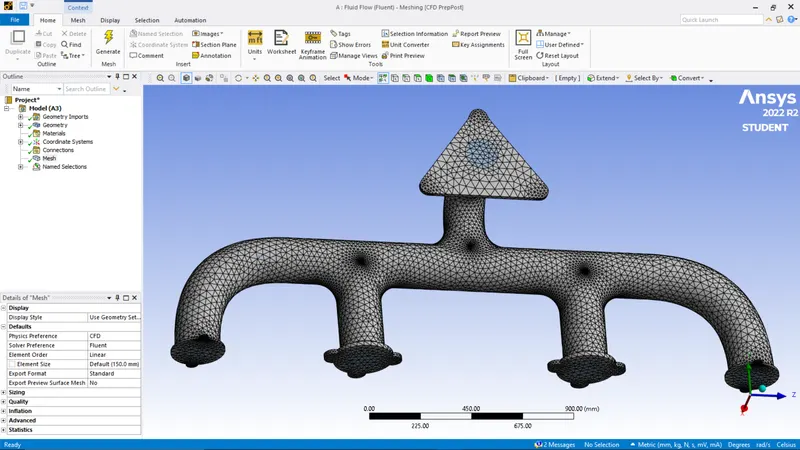
• For the given value of the mesh element, I am going to mesh the surface of the exhaust port.
• Before creating the inflation layers we have to do name selection which is for the inlet, outlet, and convection wall, inflation layers.

CREATING INFLATION LAYERS

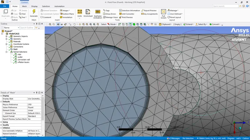
• Next, we are creating the inflation under the mesh options=>under automatic inflations=>select all the faces in chosen name selection option=>under named selection=>inflation layer=> inflation option=>first layer thickness(0.5m)=>under number of layers(5)=>select update the mesh. Inflation layers are shown below image.

SETUP AND SOLUTIONS:

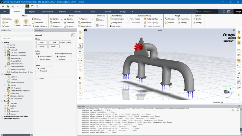
• In this, we provide fundamental physics, types of solver, boundary conditions, and type of turbulent model used.
• Initially, we go for the SOLVER option here we are the type of solver used is PRESSURE BASED SOLVER (M<0.3), and since the variable is not varying with respect to time select the STEADY STATE option.
• In the following step in for the PHYSICS, the window selects the VISCOUS option we get the window opened up. Here we are selecting the type of viscous model which is a TURBULENT model (k-omega). Since we have to calculate the temperature energy is turned on.
• In cell zone conditions we change the solid structure(In this simulation we consider the solid structure as ALUMINIUM with a heat transfer coefficient of 20 W/mK ) from the fluid domain to the solid domain.
• We are giving the BOUNDARY conditions for the inlet velocity as 5m/s and temperature as 700K.
• The hybrid method is used for initialization.
• Finally, we are obtaining the graph heat transfer coefficient with respect to temperature and contour plots.

RESULTS

• Then for obtaining the contour plot for variation of temperature and velocity, Under PLANE we do a COLOR option to change the VARIABLE option.

SIMULATION PERFORMED FOR 150mm MESH SIZE

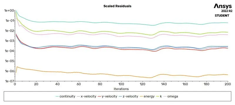
The model got converged for 200 iterations and the results are stated below

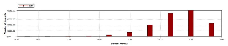
mesh quality

Scaled residual plot

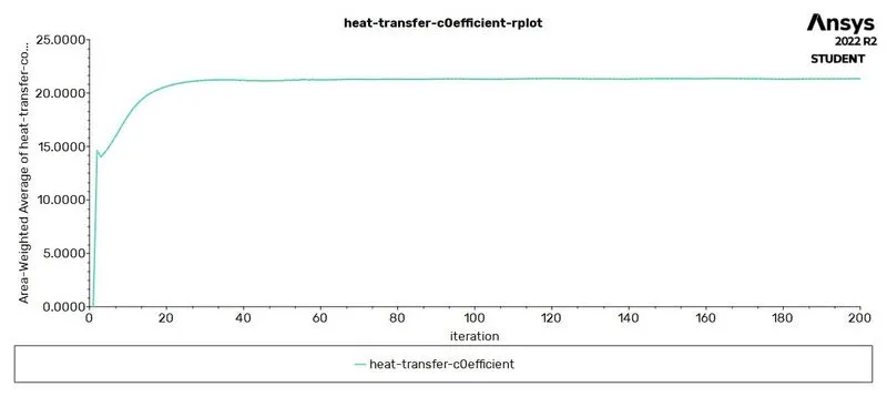
Averaged heat transfer coefficient plot

temperature contour

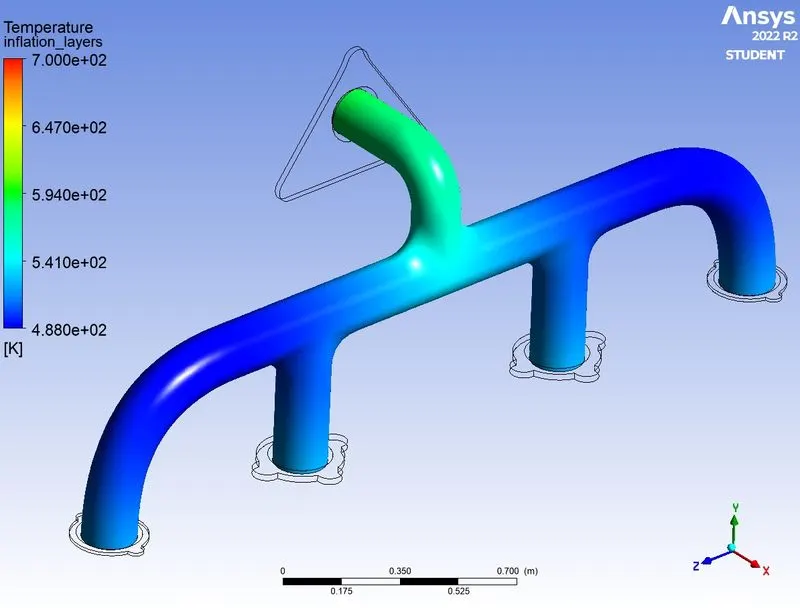
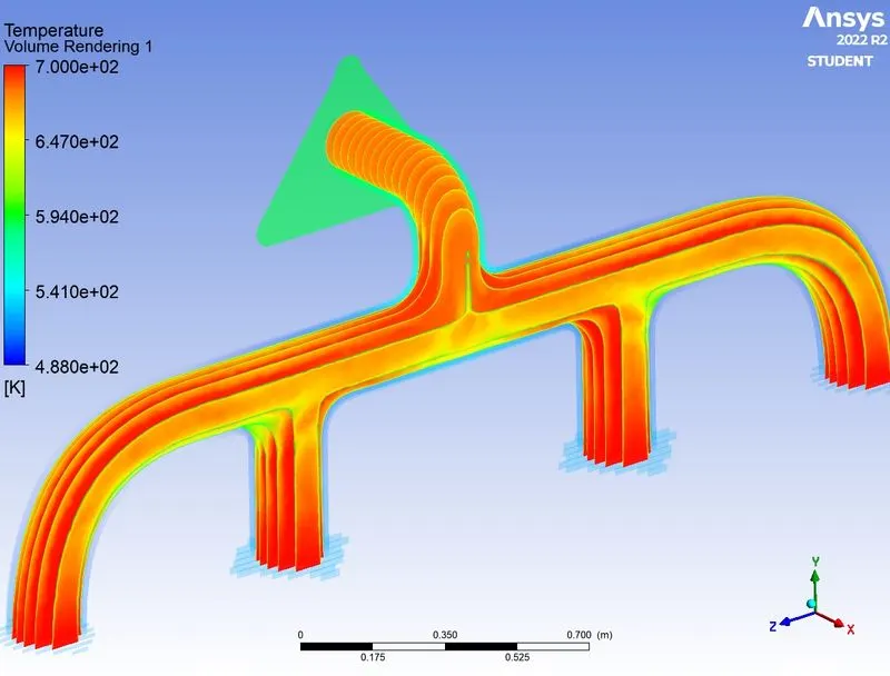
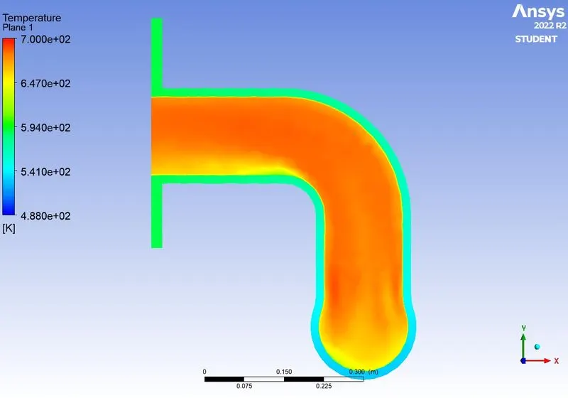
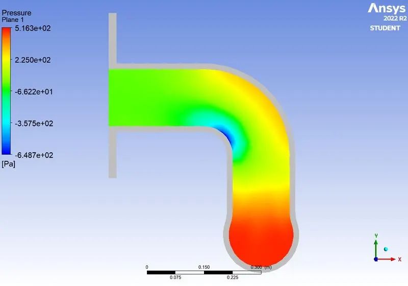
pressure contour

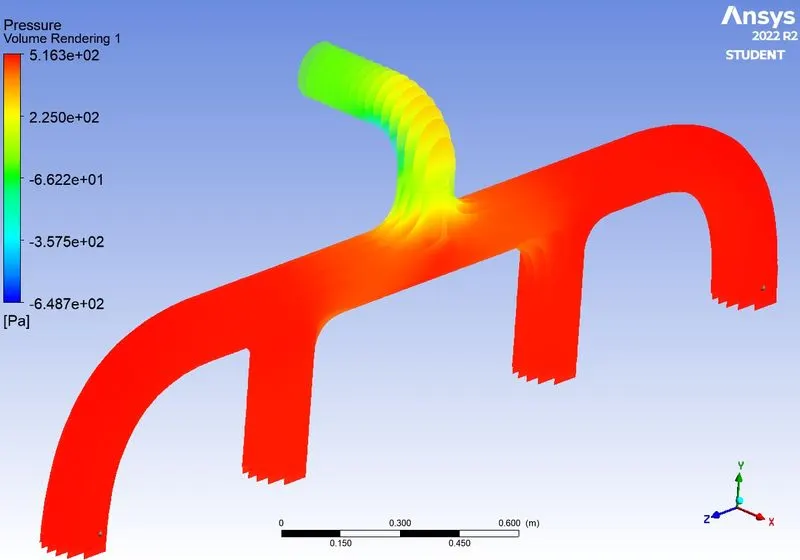
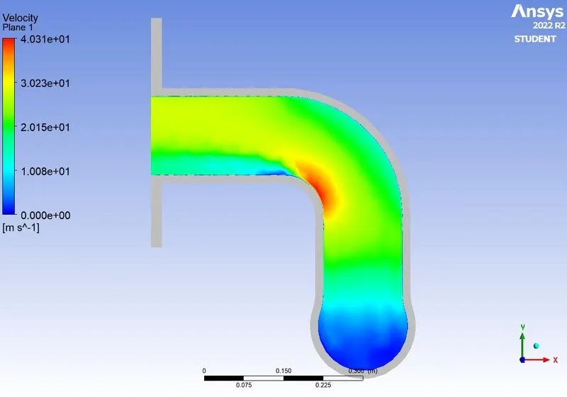
velocity contour

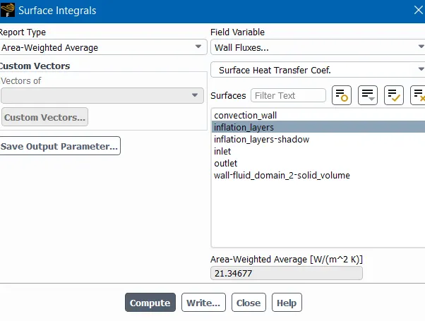
The average heat transfer coefficient is 21.34W/m^2K

CONCLUSIONS

By obtaining the heat transfer coefficients for both numerical and simulation we got to know those heat transfer coefficients are almost the same which is 21.34 W/m^2K. Also, 150mm is the ideal mesh element size for meshing.