Week 4 - CHT Analysis on Exhaust port
EXHAUST PORT SIMULATION
INTRODUCTION
Heat transfer is the branch of thermal engineering that concerns the generation, use, conversion and exchange of thermal energy (heat) between physical systems. Heat transfer is classified into various mechanisms, such as thermal conduction, thermal convection, thermal radiation, and transfer of energy by phase changes. Engineers also consider the transfer of mass of differing chemical species, either cold or hot, to achieve heat transfer. While these mechanisms have distinct characteristics, they often occur simultaneously in the same system.
Heat conduction, also called diffusion, is the direct microscopic exchange of kinetic energy of particles through the boundary between two systems. Heat convection occurs when bulk flow of a fluid (gas or liquid) carries heat along with the flow of matter in the fluid. Thermal radiation occurs through a vacuum or any transparent medium (solid fluid or gas) by transfer of energy through photons in electromagnetic waves.
CONJUGATE HEAT TRANSFER
Conjugate Heat Transfer (CHT) analysis deals with the study of heat transfer between solid and fluid domains by exchanging thermal energy at the interfaces between them, using a model based on a strictly mathematically stated problem.
In solids, conduction often dominates whereas in fluids, convection usually dominates. Conjugate heat transfer corresponds with the combination of heat transfer in solids and heat transfer in fluids.
Typical applications of this analysis type exist as, but are not limited to, the simulation of heat exchangers, cooling of electronic equipment, and general-purpose cooling and heating systems.
WHY CHT?
Heat transfer in solids is mainly due to conduction, as described by Fourier's law defining the conductive heat flux, q, proportional to the temperature gradient:  .
.
Due to the fluid motion, three contributions to the heat equation are included:
- The transport of fluid implies energy transport too, which appears in the heat equation as the convective contribution. Depending on the thermal properties on the fluid and on the flow regime, either the convective or the conductive heat transfer can dominate.
- The viscous effects of the fluid flow produce fluid heating. This term is often neglected, nevertheless, its contribution is noticeable for fast flow in viscous fluids.
- As soon as a fluid density is temperature-dependent, a pressure work term contributes to the heat equation. This accounts for the well-known effect that, for example, compressing air produces heat.
Conjugate heat transfer helps us to integrate the effects of thermal conduction and thermal convection by monitoring the heat exchange process at the interface of the solid and fluid. This helps us to understand and capture the physics involved in the effective heat transfer in any system. This makes CHT analysis important in designing systems like heat exchangers, heat sinks, etc.
A CHT model, based on a strictly mathematically stated problem, describes the heat transfer between a body and a fluid flowing over or inside it as a result of the interaction of two objects. The physical processes and solutions of the governing equations are considered separately for each object in two subdomains. Matching conditions for these solutions at the interface provide the distributions of temperature and heat flux along the body–flow interface, eliminating the need for a heat transfer coefficient. Moreover, it may be calculated using these data.
APPLICATIONS
Starting from simple examples in the 1960s, the conjugate heat transfer methods have become a more powerful tool for modeling and investigating nature phenomena and engineering systems in different areas.
Typical applications incluce -
- Designing effective coolers, heaters or heat exchangers
- Designing heat sinks in electronic packages
- Thermal analysis of turbine vanes
- Aerospace
- Nuclear reactors
- Thermal goods treatment
- Food processing
- Atmospheric/thermal interactions in meteorology
- Procedures in medicine
AIM
- To simulate the flow the flow of air through the exhaust port of a 4 cylinder inline engine
- To calculate the value of heat transfer coefficient on the internal solid surface using appropriate turbulence model
- To plot the temperature contour and velocity profiles in the exhaust port
METHODOLOGY
To find out the HTC for an Exhaust Port and conduct theral analysis, the following procedure was followed:
- Baseline simulation - Setting up simulation without regard for y+ value
- Choosing the right y+ value - Considering 3 cases to determine the value of first layer thickness that gives accurate results according to the turbulence model selected.
- Considering the best case for final simulation and plotting of contours and HTC.
BASELINE SIMULATION
Geometry
The geometry of the exhaust port is as shown in the figure with 4 inlets and 1 outlet.
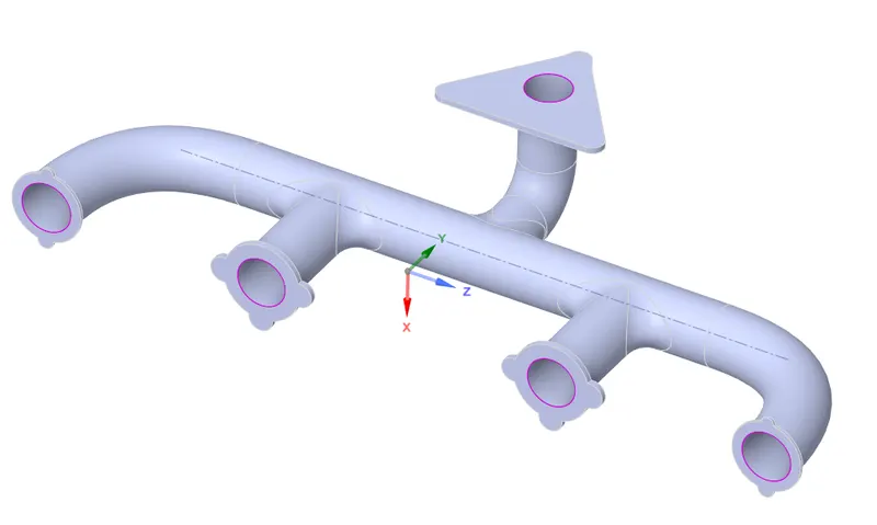
Inlet radius: 83.05mm
Outlet radius: 75mm
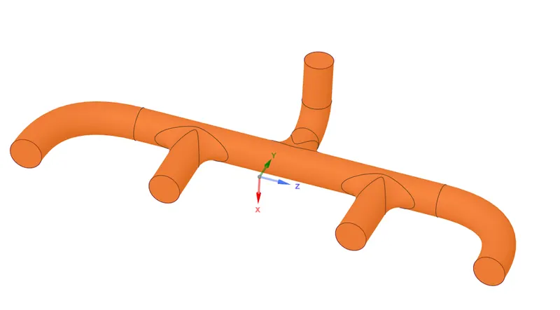
A volume extract was prepared to denote the fluid volume inside the exhaust port. Shared topology was enabled to get a consistent mesh in the meshing stage.
Meshing
A standard mesh was generated for the baseline simulation without any regard for the y+ value, initially. This was done only to first check if the setup is generating an appropriate solution.
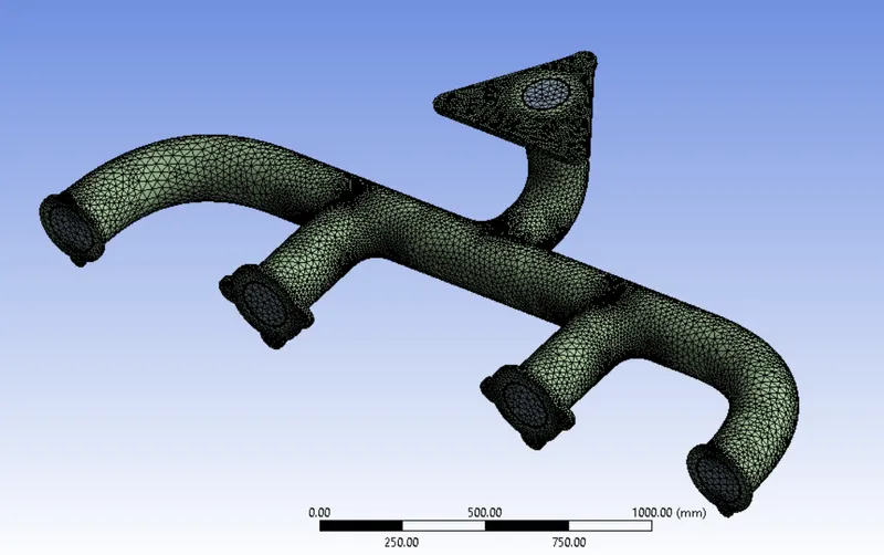
The methods used were
Inflation - 5 inflation layers with a total thickness of 5mm were used for the solid-fluid interface.
Body sizing - This was used for the solid body of exhaust port with an element size of 10mm.
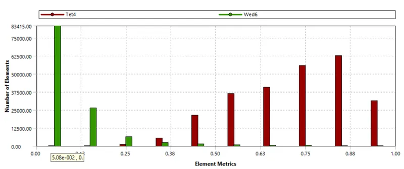
Minimum mesh quality was not less than 5%. Thus, the mesh is acceptable.
Setup
The standard k-epsilon turbulent model was used. The model would also solve for the energy equation, since temperature calculations are critical for a CHT analysis.
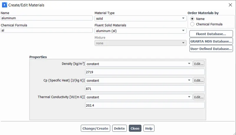
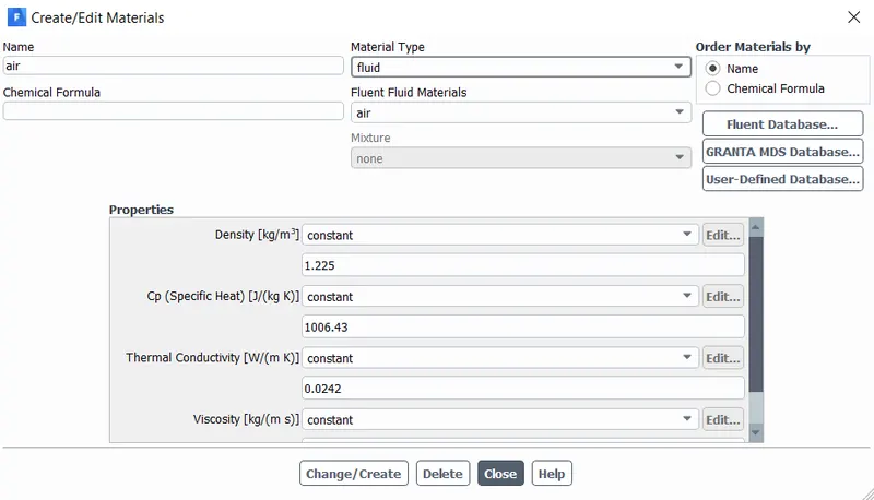
Materials used were: Air for fluid and Aluminium for solid.
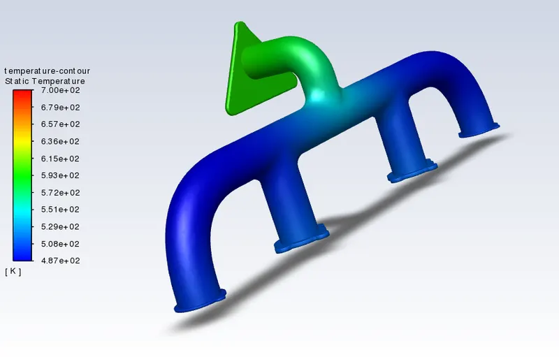
Inlet air - 5m/s at 700K
Convective heat transfer coefficient for outer wall - 20W/m^2.K
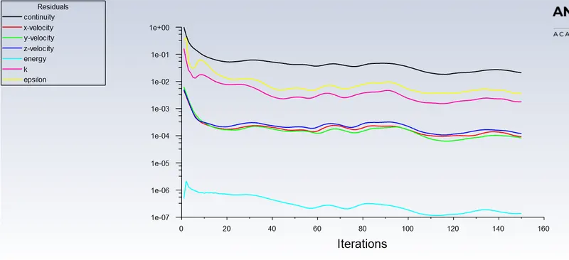
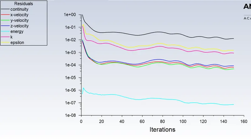
Hybrid initialization, solution run for 150 iterations.
Solution
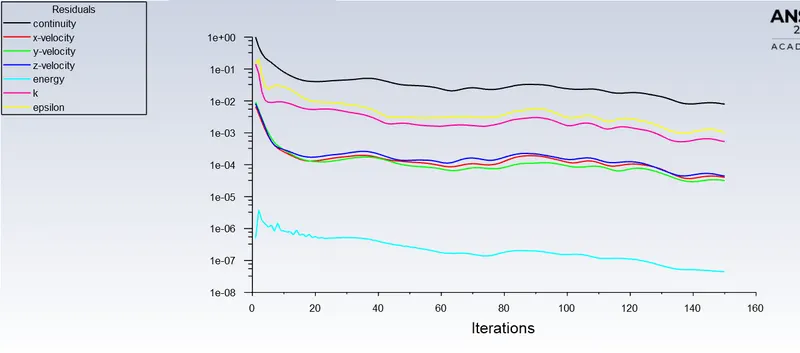
Residuals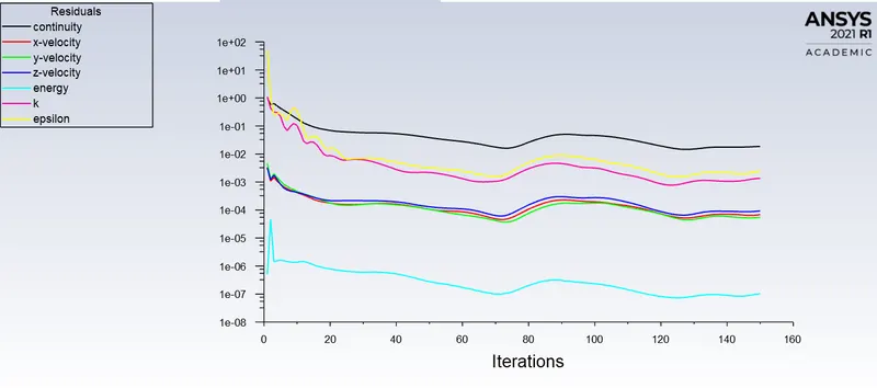
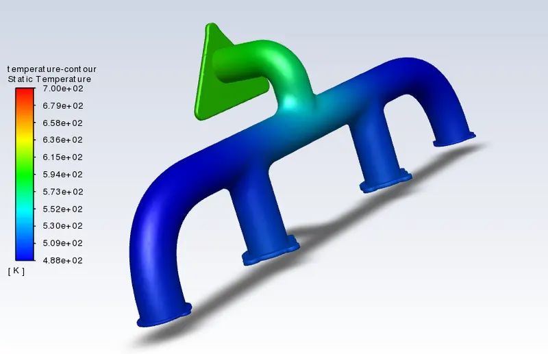
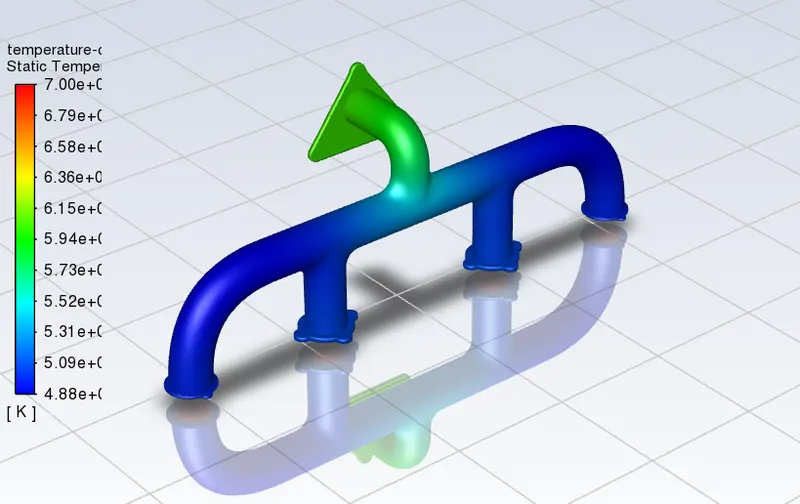
Temperature contour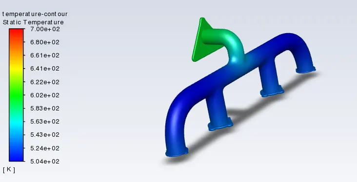
Velocity profile (XY Plane - Near outlet)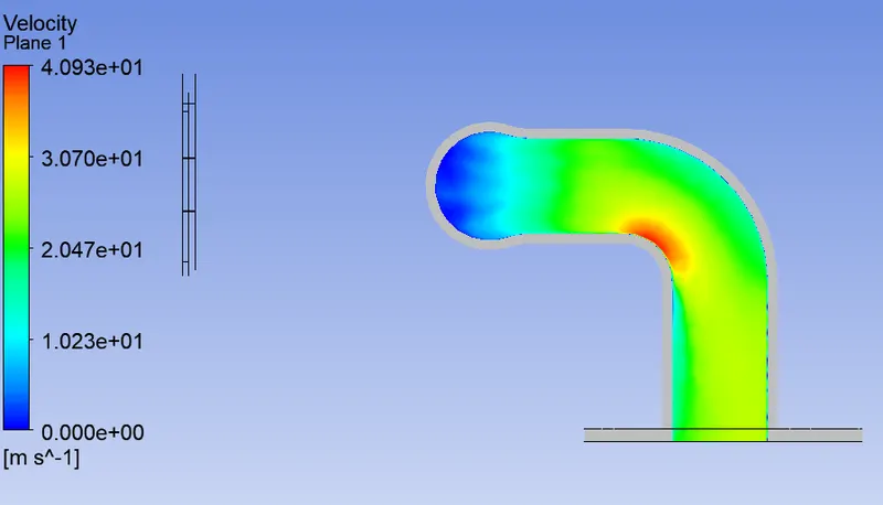
Streamlines (Velocity)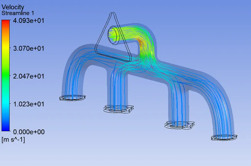
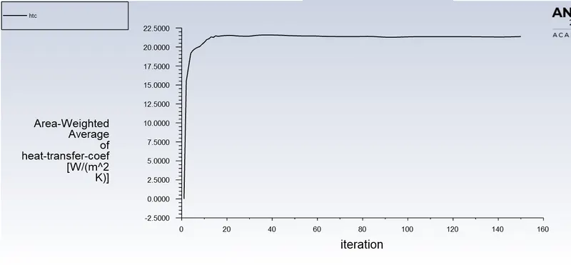
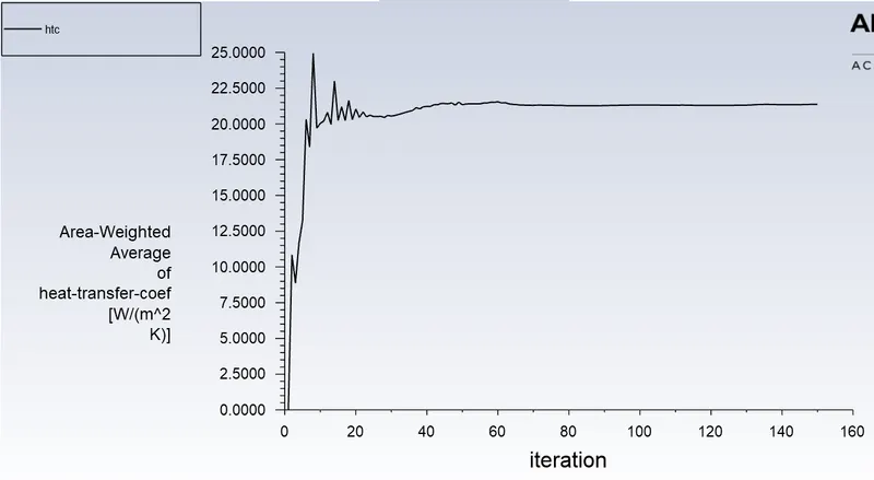
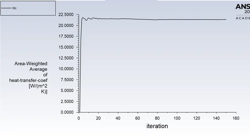
Average Surface Heat Transfer Coefficient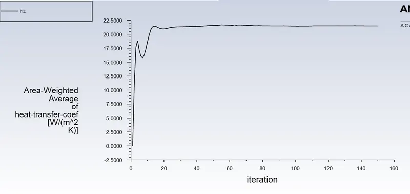
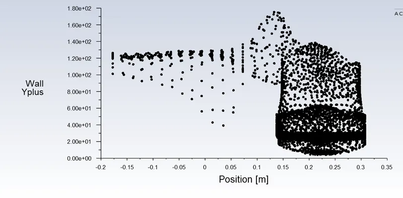
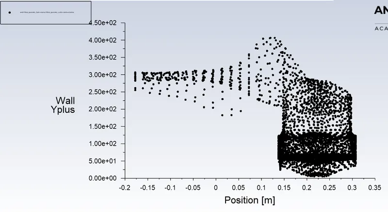
Plot: Distribution of Y+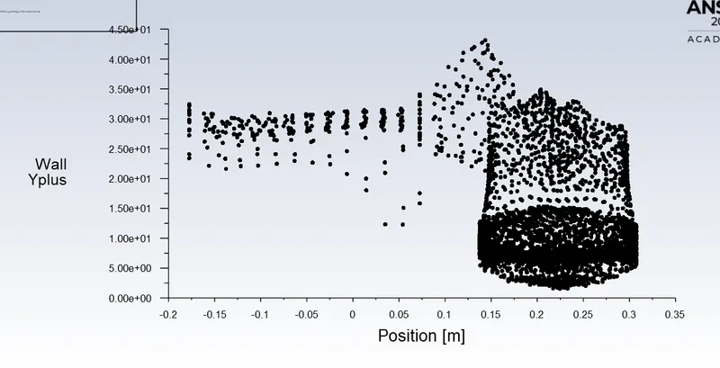
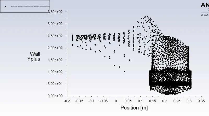
The above plot shows the distribution of cells over a range of y+ values. Most of the cells have a y+ value in the range 5-30, which is the buffer region. This is something we need to avoid. Since the chosen turbulent model is "k-epsilon standard" model, we need the y+ values of the cells in the range of 30-300. This, in the next part of this project, the simulation will be carried out for different values of y+ and its corresponding value of first layer thickness (given in the inflation layer), and the y+ value giving a suitable XY plot having most cells in the 30-300 range will be selected for plotting the streamlines, velocity profiles and HTC.
3 CASES OF Y+ VALUES
Case 1: y+ of 50, y= 2.78mm
Case 2: y+ of 100, y= 5.56mm
Case 3: y+ of 120, y=6.67mm
From the above 3 cases, we can see that with a y+ of 50 (y=2.78mm), a vast majority of the cells lie in the buffer region. This may give us inaccurate results.
Y+ values of 100 (y=5.56mm) and 120 (y=6.67mm), both generate boundary cells that are predominantly in the range of 30-300, which is the desired range for the turbulent model used (standard k-epsilon).
However, a y+ value of 100 (y=5.56mm) gives a much better distribution of the cells in the desired range for the standard k-epsilon turbulent model. So, we can use a first layer thickness of 5.56mm and generate results from the same.
BEST CASE: Y+ 100 (PLOTS AND CONTOURS)
The geometry and setup are going to be the same as in the baseline simulation. However, the mesh can be refined further by decreasing the element size of the body sizing method used on the body of the exhaust port.
The element size will be reduced to 7mm.
Residuals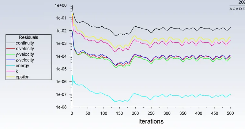
Temperature contour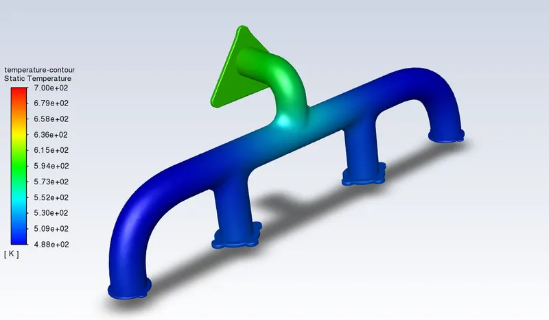
Velocity profile (XY Plane - Outlet)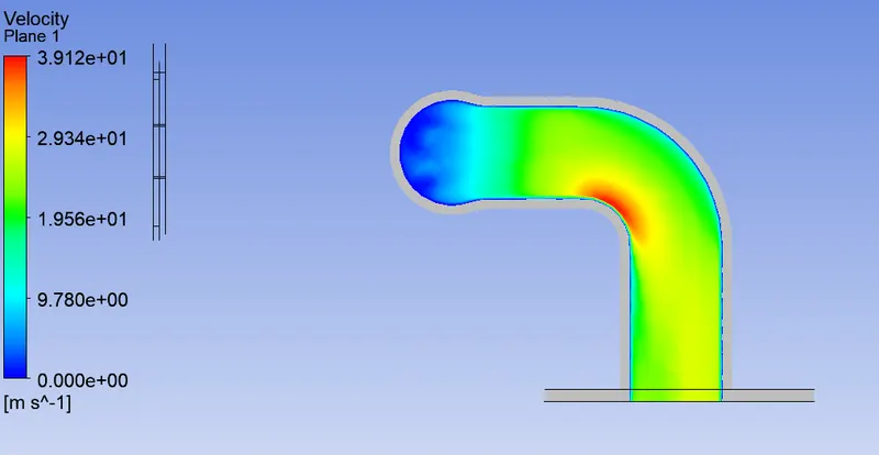
Velocity profile (YZ Plane - Inlets)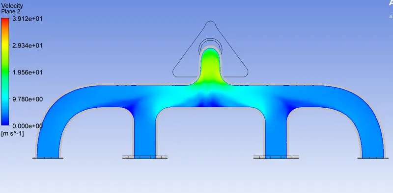
Streamlines (Velocity)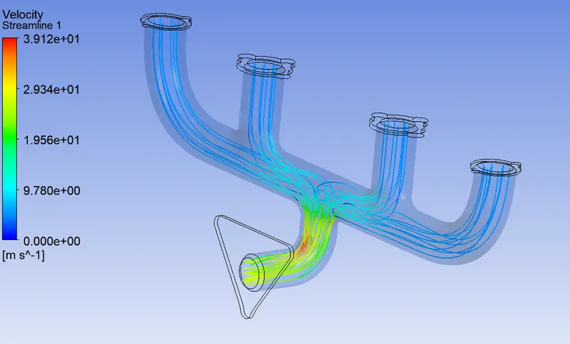
XY Plot: Y+ value vs position 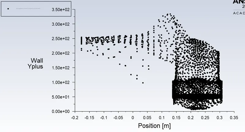
Surface heat transfer coefficient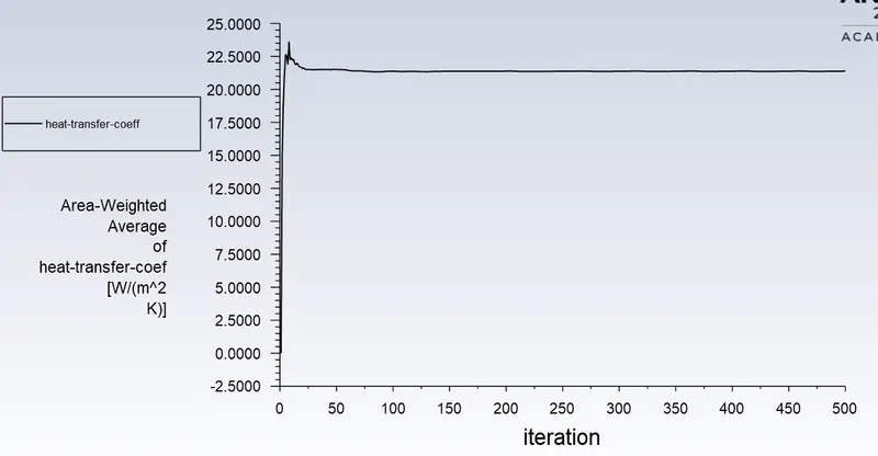
VERIFICATION
The verification of any conjugate heat transfer analysis is done by finding an analytical solution to the problem. This is done using the following relation:
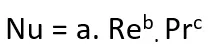
Nu - Nusselt number
Re - Reynolds number
Pr - Prandtl number
a,b,c - Dimensionless number based on experimental conditions
The value of a,b,c depends totally on experimental conditions. However, these values for standard shapes have been derived using experiments.
Since it is not a standard shape, the validation of the Exhaust Port Simulation can only be done by carrying out physical experiments and finding out the values of a, b, and c to further calculate the surface heat transfer coefficient.
ACCURACY OF HEAT TRANSFER COEFFICIENT
The accuracy of heat transfer coefficient depends mainly on the following factors:
- Value of y+
As we know, Q= hA(Tsurface - Tref), this equation is important for surface heat transfer coefficient. The term Tref (Reference temperature), depends on the first layer thickness for wall heat transfer coefficient. As the y+ value changes, it changes the first layer thickness, which in turn, affects the accuracy of the HTC, as the reference temperature used for calculation changes. - Turbulence model used
The turbulence model used also affects the value of heat transfer coefficient as HTC is sensitive to the wall functions used. For example, since a k-epsilon model solves away from the wall and k-omega model solves near the wall, both may generate different values of heat transfer coefficient.
CONCLUSION
Heat transfer in solids and heat transfer in fluids are combined in the majority of applications. This is because fluids flow around solids or between solid walls, and because solids are usually immersed in a fluid. An accurate description of heat transfer modes, material properties, flow regimes, and geometrical configurations enables the analysis of temperature fields and heat transfer. Such a description is also the starting point for a numerical simulation that can be used to predict conjugate heat transfer effects or to test different configurations in order, for example, to improve thermal performances of a given application.
Choosing the right turbulence model and appropriate y+ value is extremely critical to conducting a CHT analysis and getting accurate value of Heat transfer coefficient.