Week 4.1 - Solving second order ODEs

AIM

Solving Second Order ODEs using MATLAB

THEORY

ODE is used to describe the transient behaviour of a system.

Example;

PENDULUM

The path of the pendulum depends on Newton’s second law. ODE representing the equation of motion of a simple pendulum with damping is expressed as below:

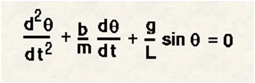
In the above equation,

• g = gravity in m/s²,
• L = length of the pendulum in m,
• m = mass of the ball in kg,
• b = damping coefficient.

Ode45

Ode45 is a function in Matlab that solves ordinary or partial differential equations using a numerical method – 4^th order Runge Kutta method.

To solve an ODE, we have to integrate and solve for the variable. Assuming we have an ode du, we would solve for u by integrating du provided some limits of integration. However, rather than direct integration, we can use a numerical solver, by discretizing the equation, that is, we convert the ODE into a linear equation and then solve this equation to approximate the solution.

How ode45 works

The function ode45 takes 3 inputs. The 3 inputs are th function to be integrated, the time span, and the initial conditions.

The function can be provided in the form of an anonymous function,

[t,results] = ode45(@(x) x^2, tspan, y0)

Here, we are saying that we don’t know the value of x and that x is an input to the anonymous function that we have defined here. This is equivalent to defining a function that takes the input of x and gives the output of x^2.

The function can also be defined as a separate function. This function must take at least 2 inputs, which should be t and y, apart from other arguments, where t would be the current time and y would be the value of the function at the previous time step.

Assuming we have a function ode, the function must be defined as,

function [output] = ode(t,y,args)

where args refer to any other arguments that the function may take.

This function must then be input to ode45 as

[t,results] = ode45(@(t,y) ode(t,y,args), tspan, y0)

This is necessary to tell the function which arguments of the function are to be found by the solver.

As mentioned above, the RK method is a first-order ODE solver and hence, so is ode45. Thus, any ODE to be integrated by ode45 must be provided as a set of first-order ODEs.

MAIN CODE

% ODE solution for Pendulum %
close all
clear all
clc

% Inputs
l = 1; % in meters
m = 1; % in kg
b = 0.05; % damping coefficient
g = 9.81; % gravity m/s^2

% Initial Conditions
theta_0 = [0;3];

% Time Duration
t_span = linspace(0,20,500);

% Pendulum ODE = diff(theta,t,2) + (b/m)*(diff(theta,t)) + (g/l)*sind(theta);

% ODE Solution 
[t,results] = ode45(@(t,theta) ode_func(t,theta,b,g,l,m),t_span,theta_0);

% Plot 
figure(1)
plot(t,results(:,1)) % displacement
hold on
plot(t,results(:,2)) % velocity
xlabel('Time')
ylabel('Plot')

% Animation
ct = 1;
for i = 1:length(results(:,1))

    figure(2)
    clf;

    % Pendulum Design drawn
    x0 = 0;
    y0 = 0;

    x1 = sin(results(i,1));
    y1 = cos(results(i,1));

    plot([-1 1], [0 0]);
    hold on 
    line([x0 x1], [y0 -y1]);
    plot(x1,-y1,"-o",'MarkerSize',30,'MarkerFaceColor','m' );
    grid on
    axis([-1.5 1.5 -1.5 0.5]);
    title('Pendulum Animation')
%     pause(0.1)

    % Capture current figure using getframe command
    M(ct) = getframe(gcf);
    ct = ct + 1;  % Loop Counter

end

% Stiching all the frames in the M array to create an animation
movie(M)

% creating a uncompressed file called pendulum.avi and assigning it to
% variable videofile
videofile = VideoWriter('pendulum.avi','Uncompressed AVI');

open(videofile)
writeVideo(videofile,M)
close(videofile)

FUNCTION CODE

% function to solve Pendulum ODE using Range-Kutta Method
% ode45

function [dtheta_dt] = ode_func(t,theta,b,g,l,m)

theta1 = theta(1);
theta2 = theta(2);
dtheta1_dt = theta2;
dtheta2_dt = -(b/m)*theta2 - (g/l)*sin(theta1);
dtheta_dt = [dtheta1_dt; dtheta2_dt];

end

OUTPUT

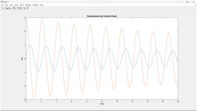
Graph

• Displacement (RED) & Velocity (BLUE) vs. Time

Animation

https://youtu.be/uNpMM9yZxhw