Week 5 - Curve fitting

CURVE FITTING – Python

OBJECTIVE

• How to change the experimental data into a mathematical equation.
• Ways to measure the goodness of fit
• To fit Cp data according to the given Cp vs temperature data file

THEORY

Curve Fitting

It is one of the techniques of data analysis to validate and find the mathematical relation between the experimental data (x and y). The curve fitting process is used to relate the x and y data by assuming the polynomial equation.

Any experimental data includes,

• Dependent variable (depends on other variables)
• Independent variable (depends on no other variable)

Example:

Considering a linear polynomial, y = ax + b

Where,

y – Specific heat (‘dependent variable’ since it depends on temperature)

x – Temperature (‘independent variable’)

a & b – Coefficients

Cubic Polynomial Fitting

Curve fitting is done by using a cubic polynomial equation.

Cp = aT³ + bT² + cT + d

It forms the cubic fitting. It is suitable for non-linear data.

CODE EXPLANATION

• Import modules
• Load the file in the python platform and plot the experimental data
• Assume the degree of polynomial respective to the data
• Calculate the respective coefficients
• Find the predicted ‘Y’ data and fit for the original data curve

Loading and extracting the data

The data extraction is done using the ‘open’ command which gets the lines in read mode. The values extracted are stored in the arrays as ‘temperature’ and ‘cp’.

Calculation of coefficients

‘curve_fit’ – It is an inbuilt command which helps to find the coefficients of the polynomial equation for the given degree. If the degree of the polynomial is ‘n’, then the ‘curve_fit’ command will return ‘n+1’ coefficients.

Output from the Main code statement

‘popt’ – The coefficients are stored in the ‘popt’.

‘pcov’ – It is a statistical term which contains a covariance matrix.

Finding the predicted values

New predicted cp is further calculated by putting the values of coefficients, and temperature in the polynomial equation.

• predicted_cp = func(np.array(temperature), *popt)

Here ‘func’ can be linear or cubic for the type of polynomial equation we are examining.

np.array(temperature) depicts all the values of the temperature which were extracted from the data file are passed in the function.

*popt passes all the coefficients of the polynomial equation in the function.

CODE

# CURVE FITTING

# importing useful modules
import numpy as np
import matplotlib.pyplot as plt
from scipy.optimize import curve_fit

# Reading thermodynamic data file
def read_file():
    temperature = []
    cp = []
    for line in open('data', 'r'):
        values = line.split(',')
        temperature.append(float(values[0]))
        cp.append(float(values[1]))
    return [temperature, cp] 

# Curve fit function (Linear Polynomial)
def linear(t, a, b):
    return a*t + b

# Main Program
# function statement to call and read the data file
temperature, cp = read_file()
# function to curve fit data 
popt, pcov = curve_fit(linear, temperature, cp)
predicted_cp = linear(np.array(temperature), *popt)

# Plot
plt.figure(1)
plt.plot(temperature, cp, color = "blue", linewidth = 3)
plt.plot(temperature, predicted_cp,, linewidth = 3)
plt.legend(['Actual data', 'Linear Curve fit'])
plt.xlabel('Temperature [K]')
plt.ylabel('Cp')
plt.grid()
plt.show()

# Curve fit function (Cubic Polynomial)
def cubic(t, a ,b, c, d):
    return a*pow(t,3) + b*pow(t,2) + c*t + d 

# Main Program
# function statement to call and read the data file
temperature, cp = read_file()
# function to curve fit data 
popt, pcov = curve_fit(cubic, temperature, cp)
predicted_cp = cubic(np.array(temperature), *popt)

# Plot
plt.figure(2)
plt.plot(temperature, cp, color = "blue", linewidth = 3)
plt.plot(temperature, predicted_cp,, linewidth = 3)
plt.legend(['Actual data', 'Cubic Curve fit'])
plt.xlabel('Temperature [K]')
plt.ylabel('Cp')
plt.grid()
plt.show()

OUTPUT

Linear Curve Fit

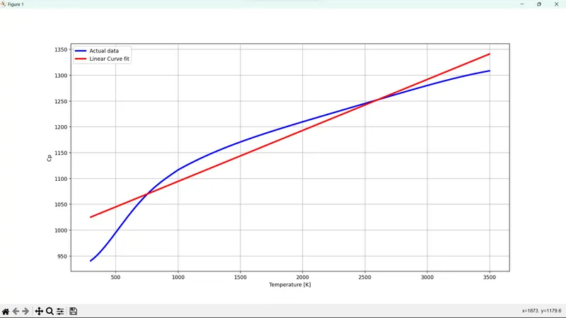
We can notice that the linear curve fit does not fit in the data provided. So this method can here be regarded as a bad fit.

Cubic Curve Fit

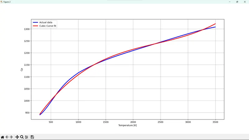
The cubic polynomial approach fits much better with the actual data curve. This method is a good fit.

GOODNESS OF FIT

It is a measure of the fitness of the curve for the given data and there are four different methods to calculate the goodness of fit as shown,

• SSE (Sum of squares due to error)
• RMSE (Root mean square error)
• R_square
• Adjusted R_square

Among the four methods of fitness calculation, the R_square value is the best method of finding the goodness of fit. Since the R_square value is an absolute quantity (ranges between 0 to 1), the remaining SSE and RMSE are relative quantities.