Week 3 - Solving second order ODEs

Solving Second Order ODE Using PYTHON

OBJECTIVE

• To create a simulation of simple pendulum with python as a solution for second-order ODE with damping.

THEORY

ODE is used to describe the transient behavior of a system.

Example;

PENDULUM

The path of pendulum depends on the Newton’s second law. ODE representing the equation of motion of a simple pendulum with damping is expressed as below:

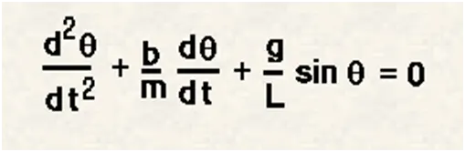
In the above equation,

• g = gravity in m/s²,
• L = length of the pendulum in m,
• m = mass of the ball in kg,
• b = damping coefficient.

CODE EXPLANATION

Python code first starts with importing all the required modules. Then the code approaches towards the problem by stating the input constants like, damping coefficient, string length, mass of pendulum etc. Next time is bounded for which the pendulum ode is solved. A function is stated where the derivative equations for the solved pendulum ODE are provided. The ODE is solved with the help of ‘odeint’ function which solves a system of ordinary differential equations using Isoda from the FORTRAN library odepack. After solving the equations, plotting part is done. At last code for creating numerous clips are created in sequential order so that they can be easily stitched to form a gif.

MAIN CODE

# 2nd oder ODE solution using Python
# Pendulum with damping ODE 

import numpy as np
from scipy.integrate import odeint
import math
import matplotlib.pyplot as plt


# Problem Constant
b = 0.5  # damping coefficients
g = 9.81 # in m/s2
l = 1    # string length
m = 1.5  # mass of pendulum

# Intital condition
theta_0 = [0,math.pi/2]

# Input for time 
t = np.linspace(0,10,150)

# Function 
def pendulum(theta,t,b,g,l,m):
    theta1 = theta[0]
    theta2 = theta[1]
    dtheta1_dt = theta2
    dtheta2_dt = -(b/m)*theta2 - (g/l)*math.sin(theta1)
    dtheta_dt = [dtheta1_dt,dtheta2_dt]
    return dtheta_dt

# solving ODE 
theta = odeint(pendulum,theta_0,t,args=(b,g,l,m))

# Plots
plt.plot(t,theta[:,0],"yellow")
plt.plot(t,theta[:,1],"blue")
plt.xlabel('Time')
plt.ylabel('Vectors')
plt.legend(["Angular Velocity","Angular Displacement"])
plt.title('Pendulum ODE')
plt.show()

# Animation Preparation
ct = 1
x0 = 0
y0 = 0

for i in theta[:,0]:
   x1 = x0 + (l*math.sin(i))
   y1 = y0 + (-l*math.cos(i))

   filename = str(ct) + '.png'
   ct = ct + 1

   plt.figure()
   plt.plot([-1,1],[0,0],"black") 
   plt.plot([x0,x1],[y0,y1],"blue")
   plt.plot(x1,y1,'o',markersize = '20')
   plt.xlim([-1.5,1.5])
   plt.ylim([-2,0.5])
   plt.title('Oscillating Pendulum')
   plt.savefig(filename)

OUTPUT

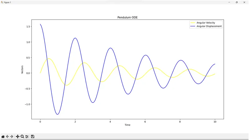
Graph

• Displacement (blue) & Velocity (yellow) vs. Time

Animation

https://youtu.be/rYCFtttBq7c