Week 2 Air standard Cycle

Otto cycle - Python

OBJECTIVE

• Introduction to IC engine and air standard cycle
• Plotting PV graph of Otto cycle using Python

THEORY

IC Engine

It is a heat engine that converts the chemical energy of fuel into mechanical energy. The chemical energy of the fuel gets converted to thermal energy through the combustion of an air-fuel mixture inside the engine. This thermal energy raises the temperature and pressure of the gases inside the engine, and then this high-pressure gas expands and makes the crankshaft rotate with the help of mechanical linkage.

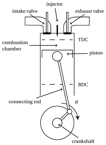
Swept volume – It is defined as the volume of oil that is swept or displaced by the actuator piston during an opening or closing cycle.

Clearance volume – The clearance volume of the engine is the volume between the cylinder head and the piston when the piston is at TDC. The ratio of this volume to the swept volume determines the compression ratio of the engine.

4-stroke engines

The top dead centre (TDC) of a piston is the position where it is nearest to the valves; the bottom dead centre (BDC) is the opposite position where it is furthest from them. While an engine is in operation, the crankshaft rotates continuously at a nearly constant speed. In a 4-stroke ICE, each piston experiences 2 strokes per crankshaft revolution in the following order.

1. Intake, induction or suction: The intake valves are open as a result of the cam lobe pressing down on the valve stem. The piston moves downward increasing the volume of the combustion chamber and allowing air to enter in the case of a CI engine or an air-fuel mix in the case of SI engines that do not use direct injection. The air or air-fuel mixture is called the charge in any case.
2. Compression: In this stroke, both valves are closed and the piston moves upward reducing the combustion chamber volume which reduces its minimum when the piston is at TDC. The piston performs work on the charge as it is being compressed; as a result, its pressure, temperature and density increase.
3. Power or working stroke: The pressure of the combustion gases pushes the piston downward, generating more kinetic energy than is required to compress the charge. Complementary to the compression stroke, the combustion gases expand and as a result their temperature, pressure and density decrease. When the piston is near BDC the exhaust valve opens.
4. Exhaust: The exhaust valve remains open while the piston moves upward expelling the combustion gases.

Air Standard Cycle

The operation of an IC engine occurs over several thermodynamic processes which are complicated tasks to evaluate. To make it simple, we consider an idealized case for the cycle, which is considered the Air Standard cycle. The air standard cycle is used to estimate engine performance.

Assumption

• The gas in the engine cylinder is assumed to be perfect gas.
• The compression and expansion process that takes place inside the engine cylinder is assumed to be adiabatic and reversible.
• The cycle is considered to be taking in a closed system with no air leaving or entering the system.

Types

• Otto cycle
• Diesel cycle
• Dual cycle
• Brayton cycle

Otto Cycle

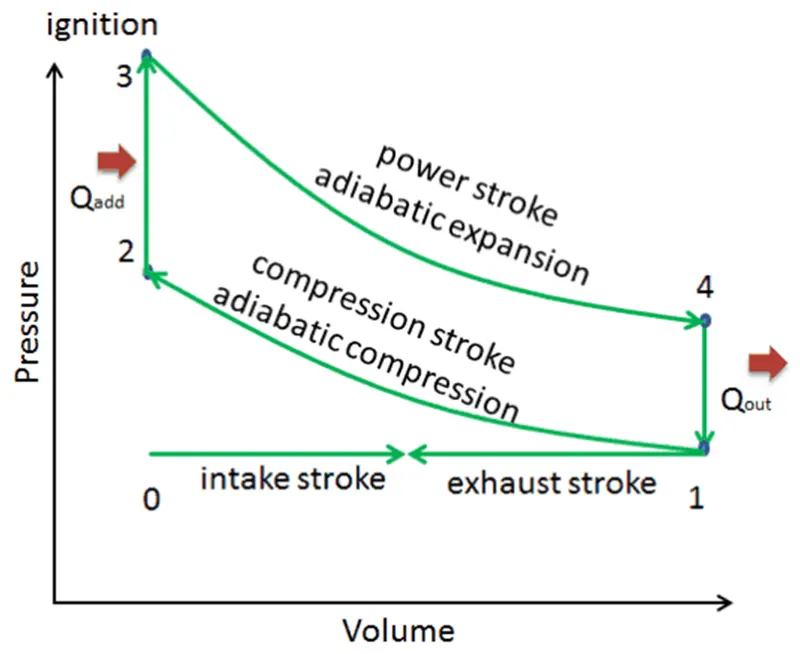
This cycle describes the functioning of a typical spark ignition piston engine. It is also known as the constant volume cycle.

PV diagram layout

Thermodynamic Relations

• PV^gamma = constant for adiabatic process
• PV = nRT

Piston Kinematics equation

• Here, V is the stroke volume
• V_c is the clearance volume
• r_c is the compression ratio
• R is the ratio of connecting rod length to crank pin radius
• `Theta` is the crank angle

CODE EXPLANATION

• Define engine geometric parameters
• Scripting the piston kinematics function
• Calculation of four state points (pressure and volume)
• Plotting the PV diagram

CODE

"""
    otto cycle simulator
"""

import math
import matplotlib.pyplot as plt

def engine_kinematics(bore, stroke, con_rod, cr, start_crank, end_crank):
    """
      Engine Kinematics function which traces the volume for expansion and compression for varying crank angles.
    """

    # Geometric parameters
    a = stroke/2
    R = con_rod/a

    # Volume parameters
    V_s = math.pi*(1/4)*pow(bore,2)*stroke
    V_c = V_s/(cr-1)

    s_c = math.radians(start_crank)
    e_c = math.radians(end_crank)

    num_value = 50

    dtheta = (e_c-s_c)/(num_value-1)

    V = []

    for i in range(0,num_value):
        theta = s_c + i*dtheta
        term1 = 0.5*(cr-1)
        term2 = R + 1 - math.cos(theta)
        term3 = pow(R,2) - pow(math.sin(theta),2)
        term3 = pow(term3,0.5)

        V.append((1 + term1*(term2 - term3))*V_c)

    return V

# inputs
p1 = 101325
t1 = 500
t3 = 2300
gamma = 1.4

# geometric parameters
bore = 0.1  # cylinder diameter
stroke = 0.1  # vertical distance in which the piston slides
con_rod = 0.15  # length of connecting rod
cr = 12    # compression ratio - ratio of volume before compression to the volume after compression

# Volume computation
v_s = (math.pi/4)*pow(bore,2)*stroke
v_c = v_s/(cr-1)
v1 = v_c + v_s  # volume before compression is the sum of swept volume(v_s) and clearance volume (v_c)

# state point 2
v2 = v_c  # v_c refers to clearance volume or volume after compression 

# p2v2^gamma = p1v1^gamma
p2 = p1*pow(v1,gamma)/pow(v2,gamma)

# p2v2/t2 = p1v1/t1 | rhs = p1v1/t1 | p2v2/t2 = rhs | t2 = p2v2/rhs
rhs = p1*v1/t1
t2 = p2*v2/rhs

# engine kinematics
V_compression = engine_kinematics(bore, stroke, con_rod, cr, 180, 0)

constant = p1*pow(v1,gamma)
P_compression = []

for v in V_compression:
    P_compression.append(constant/pow(v,gamma))

# state point 3
v3 = v2

# p3v3/t3 = p2v2/t2 | rhs = p2v2/t2 | p3 = rhs*t3/v3

rhs = p2*v2/t2
p3 = rhs*t3/v3

# engine kinematics 
V_expansion = engine_kinematics(bore, stroke, con_rod, cr, 0, 180)

constant = p3*pow(v3,gamma)
P_expansion = []

for v in V_expansion:
    P_expansion.append(constant/pow(v,gamma))

# state point 4 
v4 = v1

# p4v4^gamma = p3v3^gammma

p4 = p3*pow(v3,gamma)/pow(v4,gamma)

# p4v4/t4 = p3v3/t3 = rhs

t4 = p4*v4/rhs

# Thermal Efficiency
e = 1 - (t4 - t1)/(t3 - t2)
print(e)

# Plot
plt.plot([v2,v3],[p2,p3])
plt.plot(V_compression, P_compression)
plt.plot(V_expansion, P_expansion)
plt.plot([v4,v1],[p4,p1])
plt.xlabel('Volume(m^3)')
plt.ylabel('Pressure(Pa)')
plt.title('PV plot for Otto Cycle')
plt.legend(['constant volume heat addition','adiabatic compression','adiabatic expansion','constant volume heat rejection'])
plt.grid()
plt.show()

OUTPUT

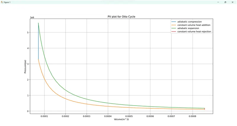
PV Plot

Thermal Efficiency

Output Value

REFERENCES

• https://www.researchgate.net/figure/The-basic-geometry-of-an-engine-cylinder-Combustion-of-fuel-and-air-in-the-combustion_fig1_325086523
• https://en.wikipedia.org/wiki/Internal_combustion_engine