Week 3 - Solving second order ODEs

Damped_Pendulum_ODE :

clear all
close all
clc

b=0.05; % Damping coefficient : constant
g=9.81; % Gravity : m/(s^2)
l=1;    % Length of cord / pendulum : m
m=1;    % Mass of ball / pendulum : Kg

% Initial condition
theta_0 = [0;3]; % Defines the 'Angular Velocity' of pendulum in [2*1] matrix with use of ';'.

% time points
t_span = linspace(0,20,500); % Defines time span and is distributed among '500 units' by using 'linspace' command.

% solve ODE
[t, results] = ode45(@(t,theta) ode_func(t,theta,b,g,l,m),t_span,theta_0);

x1 = l*sin(results(:,1)); % Defines x-coordinate of pendulum at particular value of 'time' and 'velocity'.
y1 = -l*cos(results(:,1)); % Defines y-coordinate of pendulum at particular value of 'time' and 'velocity'.

ct=1;
for i = 1:length(results(:,1))        
        x0 = 0;
        y0 = 0;          
        plot([-0.5 0.5],[0 0],'linewidth',5,'color','k') % This plot is used to create a fixed wall as hanger.
        hold on           
        plot([x0 x1(i)],[y0 y1(i)],'linewidth',2,'color','r') % This plot is used to create string of pendulum whose one end is fixed with wall and other is free.
        hold on        
        plot(x1(i),y1(i),'.','markersize',40,'markeredgecolor','b') % Here pendulum is created at particular points of 'i' on x-y coordinates by help of command 'markersize'.
        legend('Wall','Cord Length','Pendulum') % Used to properly define plots.                
        axis([-1 1 -1.2 0.4]) % Specifies only that graph area where plot is created.
        xlabel('Angular Velocity')
        ylabel('Displacement')       
        pause(0.03)        
        M(ct) = getframe(gcf);
        ct=ct+1;
end

movie(M)
videofile = VideoWriter('Damped_pendulum.avi','Uncompressed AVI');
open(videofile)
writeVideo(videofile,M)
close(videofile)

To obtain the curvature of the pendulum, firstly we defined the fixed values of the pendulum (like damping coefficient, gravity, length of cord, the mass of ball). After that the 'Initial & final value of Angular velocity as theta_0'. An array of time is defined as 't_span' with the 'linspace' command. Now equation for solving the differential w.r.t. time is defined. After that certain conditions are defined to obtain a plot for the pendulum.

ODE45 = This is a predefined Matlab function, used to find the values of differential equations.

[t,y] = ode45(odefun,tspan,y0) : t = time; y = value of differential equation; odefun = defined below; tspan = array of time; y0 = boundary comnditions

Damped_Pendulum_ODE_func :

function [dtheta_dt] = ode_func(t,theta,b,g,l,m)

theta1 = theta(1);
theta2 = theta(2);
dtheta1_dt = theta2;
dtheta2_dt = -(b/m)*theta2 - (g/l)*sin(theta1);
dtheta_dt = [dtheta1_dt; dtheta2_dt];
end

The above function is defined to obtain the values of theta required for the pendulum, curvature.

Errors occurred while creating the pendulum graph:

1. 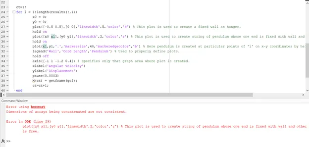This error has happened when values for creating a line on x1 & y1 coordinates are not defined in terms of 'for statement (i)'. "To avoid this error we provided x1 & y1 coordinates in terms of (i)".

2.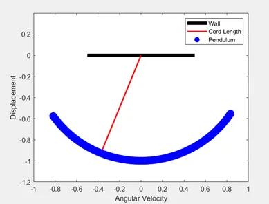 This error is obtained when the coordinates for the pendulum ball are also not defined in (i). "This error is avoided by editing command into this".

3.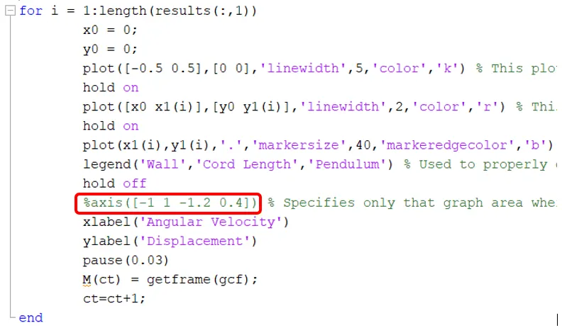 Here when "axis" is not defined then this error happens "https://youtu.be/3ZJB5I1MLG4". Here as we have not defined the axis for the graph, so it tries to fit in the screen according to the ongoing plotting of the curve.

ANIMATION PLOT: The 'YouTube' link is provided for the animation plot for "Damped Pendulum ODE"

https://youtu.be/dLyl86oh1gc