Solving second order ODEs - Simple pendulum motion
Q: Write a program in Matlab that will simulate the pendulum motion and also its animation by using the below values?
L = 1 metre, m = 1 kg, b = 0.05, g = 9.81 m/s2. Simulate the motion between 0-20 sec, for angular displacement = 0, angular velocity = 3 rad/sec at time t = 0.
Ans: A simple pendulum is a mechanical arrangement which describes the periodic motion. A simple pendulum consists of a small bob of a certain mass attached to non-extensible and negligible weight thread. Another end of a thread is fixed support. When initial conditions are provided to this system, it generates a motion called the periodic motion of a simple pendulum.
In other words, suspension of a mass with a thread and calculation of its motion.
The whole setup is represented in the following figure.
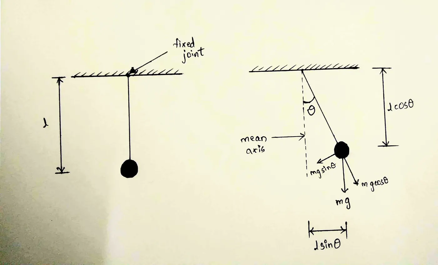
The motion of a simple pendulum with initial values are solved in MATLAB using ODE.
ODE means Ordinary Differential Equation. It is a differential equation containing one or more functions of one independent variable and derivatives of those functions. The order of an ODE is the highest derivative present in the equation.
To solve higher ODE, we need to convert it into first-order differential equations and solve it. In MATLAB, ode45 is used for solving the system.
We can also solve other problems like dampers and springs used in vehicle dynamics by this kind of method.
Syntax:
[t, y] = ode45(odefun, tspan, y0)
where tspan = [ti tf]
y0 = initial condition
tspan integrates within the limits of ti to tf.
odefun is a function of solvable expression. In this function, y0 values are taken into consideration initially and solved continuously.
Below is the ODE that represents the equation of motion of a simple pendulum:
Terms and its definitions:
b = Damping coefficient.
m = mass of the bob.
g = gravity.
L = length of the pendulum.
Angular displacement: Displacement that occurred in angles of a mass is known is Angular displacement.
Angular Velocity: The rate of change of angular displacement with respect to time is known as Angular Velocity.
Damping coefficient: The property that describes whether the object will bounce back or return energy to a system is called a damping coefficient. High damping coefficient reduces the unwanted vibrations, shock, noise and swallows the energy.
'theta' is denoted by displacement and 't' is denoted by time.
The above equation is a second-order equation and for solving we convert them into first-order differential equations.
Let us assume, θ = θ1
By derivating wrt to 't',
dθ/dt = dθ1/dt
Let us assume dθ1/dt = θ2
⇒ dθ/dt = θ2
By derivating on both sides, we get
dθ^2/dt^2 = dθ2/dt
Hence, the ODE can be written as
dθ^1/dt^2 + (b/m) * (dθ1/dt) + (g/L) * sin θ1 = 0
⇒ dθ2/dt + (b/m) * (θ2) + (g/L) * sin θ1 = 0
∴ We created 2 ODE's
- dθ1/dt = θ2
- dθ2/dt = - (b/m) * (θ2) - (g/L) * sin θ1
This is represented in the form of column matrix.
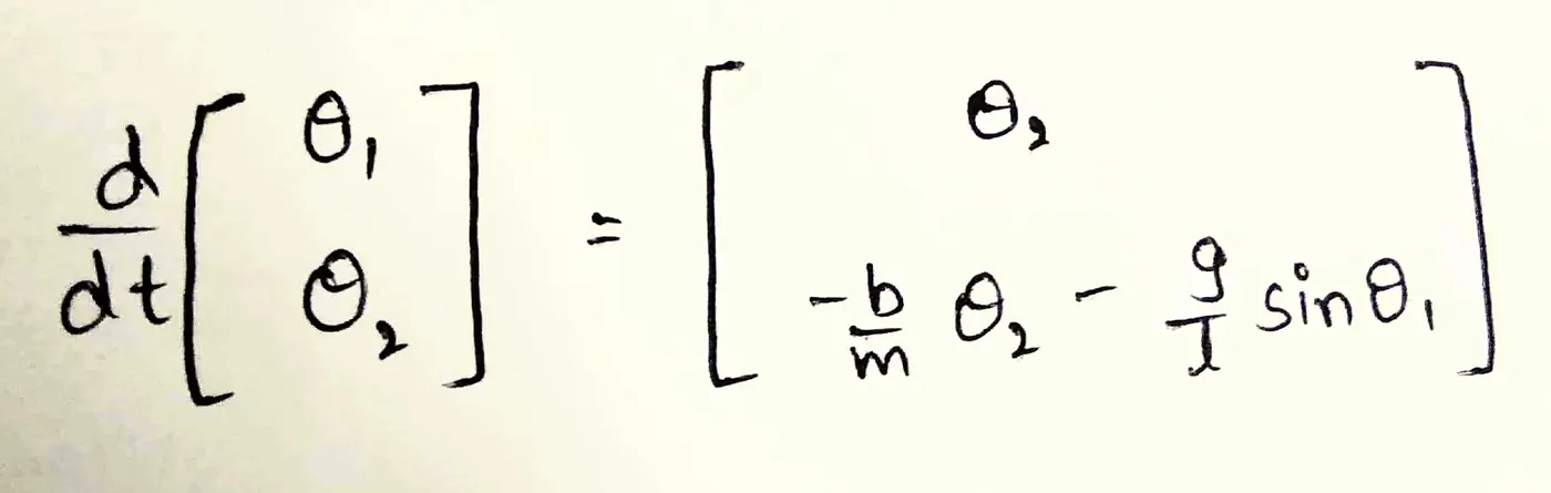
To solve this solution, we write code in two scripts. The above conversion is written in the main script and plotting is done in execution script.
Main script:
- Open MATLAB and click new script.
- Add function in the name of 'dtheta_dt'.
function [dtheta_dt] = ode_func(t, theta, b, g, l, m) - To avoid confusion while writing code, we assign theta(1) to theta1 and theta(2) to theta2.
theta1 = theta(1)
theta2 = theta(2) - Converted 2 ODE's are written in code.
dtheta1_dt = theta2;
dtheta2_dt = -(b/m) * theta2 - (g/l) * sin(tehta1) ; - Both ODE's are written in the form of a column matrix. This matrix is equal to function name 'dtheta_dt'.
dtheta_dt = [dtheta1_dt ; dtheta2_dt] ; - Therefore we get the final equation for solving ODE by combing them in a single column array.
Code for the main script:
function [dtheta_dt] = ode_funcsample(t, theta, b,g,l,m)
theta1 = theta(1)
theta2 = theta(2)
dtheta1_dt = theta2;
dtheta2_dt = -(b/m) * theta2 - (g/l) * sin(theta1);
dtheta_dt = [dtheta1_dt ; dtheta2_dt]
Execution script:
- This is the tab where the function is called and the program is run for plotting the graphs and motion.
- Open the new script and add statements as shown below.
clear all
close all
clc - Add initial values such as damping coefficient, gravity, length and mass of the bob.
b = 0.05;
g = 9.81;
l = 1;
m = 0.1; - To solve 2 ODE's we need to give initial values for displacement and velocity. The first value is given for displacement and second is angular velocity.
ini = [0 ; 5]; - Now give the value for time, initially t = 0 secs and also simulate the motion between 0 - 20 seconds. This can be given 'linspace' command with 500 values in between.
t_span = linspace(0, 20, 300) - Till now we got all the requirements for solving ODE function. Give 'ode45' statement for solving the equation.
[time, results] = ode45(@(t, theta) ode_func(t, theta, b, g, l, m), t_span, ini)
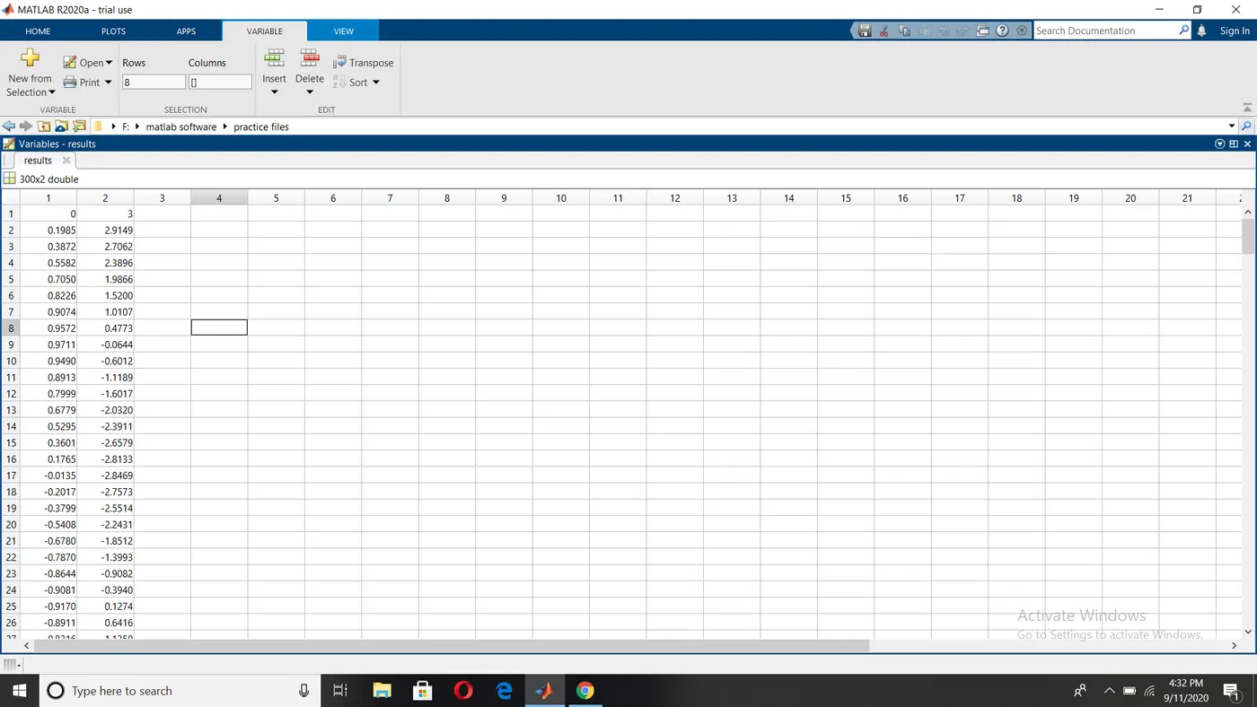
'ode45' is an inbuilt solver in MATLAB and @(t, theta) contains two main inputs of a differential equation. Later, the function 'ode_func' is defined with inputs that are needed for solving. Motion time and initial values are given respectively according to syntax. - We get two values in the single variable i.e., in results. To visible these, double click on 'results' from the workspace. You get two columns of values. The first column represents displacement and the second column represents the angular velocity.
- Plot time and results with 'plot' commands. We need to plot two lines. First one is between time and displacement and the second is between time and angular velocity.
Plot(time, results(:, 1), 'r', time, results(:, 2), 'b') - Give labels of X and Y-axis.
xlabel('time')
ylabel('results')
title('Plots of displacement and velocity wrt to time') - We need to know which curve represents displacement-time and velocity-time. We need to add 'legend' command.
legend('disp-vel', 'vel-time') - Add hold off command for stopping of intermixing of both figures.
hold off - Now, we have plot motion of a simple pendulum. For this, we need to create a 'for' loop. After running the code we get many frames for the motion. These frames are transferred into an array and created a video of the motion of a simple pendulum. Create a figure 2 and 'for' loop with a counter value 1.
figure(2)
ct = 1
for i = 1 : length(results(:,1)) - Give fixed joint coordinate as origin which can be represented by x0 and y0.
x0 = 0
y0 = 0 - The centre position of bob is given by x1 and y1.
x1 = l * sin(results(i : 1)) ;
y1 = -l * cos(results(i : 2)) ; - Plot a line where a thread is fixed.
plot([-1 1], [0 0], 'linewidth', 3, 'color', 'r') - Give a hold on command for avoiding termination of previous plot.
hold on - Plot a thread which can be given by below.
plot([x0 x1], [y0 y1], 'color', 'black') - Give a hold on command for avoiding termination of previous plot.
hold on - Now we have to create a bob. Since it is a 2D plot, we create a circle shape. This can be done using the marker and with size 20 and red colour. 'Marker' is command tool in MATLAB which is used to display text.
plot(x1, y1, 'O', 'MarkerSize', 20, 'color', 'b', 'MarkerFaceColor', 'b') - Give a hold on command for avoiding termination of previous plot.
hold on - Plot axis of a simple pendulum. We know axis should be dashed line and LineStyle is given as '--' with colour black.
plot([0 0], [0 -1.5], 'LineStyle', '--', 'color', 'black') - Give hold off command for stooping a figure.
hold off - Using pause command with a value 0.003.
pause(0.003) - Give the axis limits.
axis(-2 2 -2 1.5) - We get more figures for motion. To combine these figures, an array 'M' is given and all frames are inserted in it.
M(ct) = getframe(gcf) - Give incrementation for 'ct' value.
ct = ct + 1 ; - End the 'for' loop.
end - We have an array which contains all frames. These frames are converted into a motion i.e., into a video. The video is in AVI format.
movie(M)
videofile = VideoWriter('simple_pendulum_motion.avi', 'uncompressed AVI')
open(videofile)
WriteVideo(videofile, M)
close(videofile)
Code for execution script:
clear all
close all
clc

% input
b = 0.01;
g = 9.81;
l = 1;
m = 0.1;

% initial condition
ini = [0 ; 3]

% time points
t_span = linspace(0, 20, 300);

% solve ODE
[time, results] = ode45(@(t, theta) ode_funcsample(t,theta,b,g,l,m), t_span, ini);

%plotting

figure(1)
plot(time, results(:, 1), 'r', time, results(:,2), 'b')

xlabel('time')
ylabel('plot')
title('Plots of displacement and velocity wrt to time')
legend('disp-time', 'vel-time')
hold off

figure(2)
ct = 1
for i = 1 : length(results(:,1))

    x0 = 0;
    y0 = 0;

    x1 = l*sin(results(i,1));
    y1 = -l*cos(results(i,1));
    plot([-1 1],[0 0], 'linewidth', 3, 'color', 'r')
    hold on
    plot([x0 x1], [y0 y1], 'color', 'black')
    hold on
    plot(x1, y1, 'O', 'MarkerSize', 20, 'color', 'b', 'MarkerFaceColor', 'b')
    hold on
    plot([0 0], [0 -1.5],'LineStyle', '--', 'color', 'black')
    hold off
    pause(0.03)
    axis([-2 2 -2 1.5])
    M(ct) = getframe(gcf);
    ct = ct + 1;
end

% creating animation
movie(M)
videofile = VideoWriter('simple_pendulum_motion.avi', 'uncompressed AVI')
open(videofile)
writeVideo(videofile, M)
close(videofile)
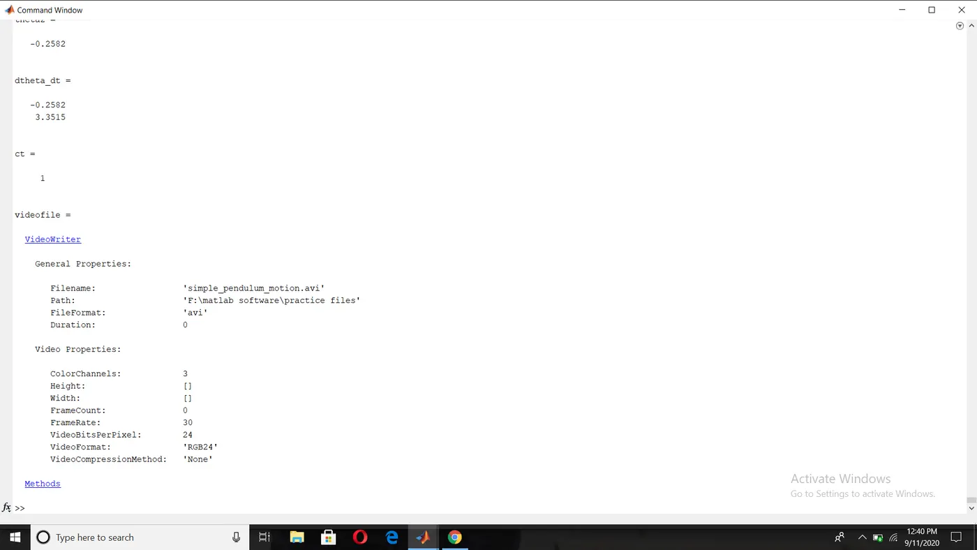
Output in the command window: Output in the command window shows values and the file details in the file manager.
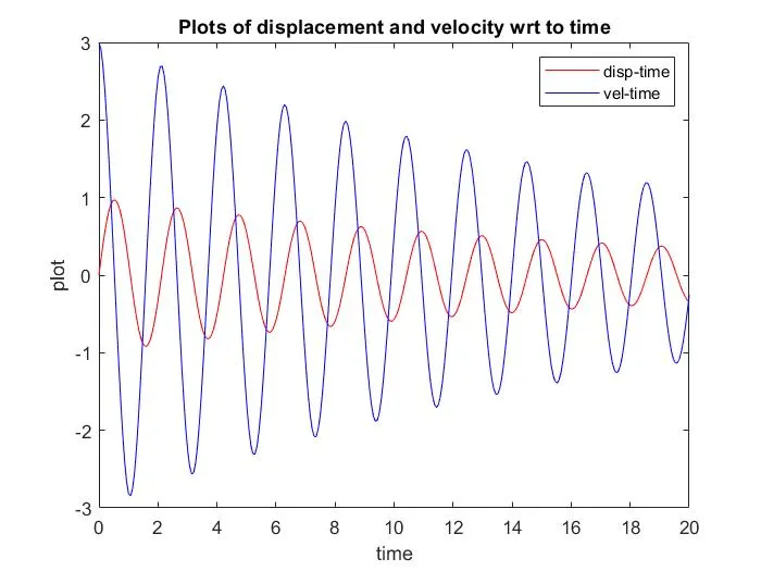
Results: First column represents displacement and second column represents velocity. We get 300x2 matrix.
Output plots of code: Two curves are represented in the time interval of 0-20 seconds. Red line represents displacemnet-time curve and blue line represents velocity-time curve.
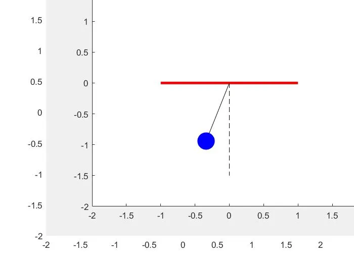
The output of figure(2): This is the figure we get when the whole program is run.
Link for the motion of a simple pendulum:
The motion of a simple pendulum using MATLAB
Points to remember:
- In main script, file name and function name should be same.
- Both script files should be in the same directory.
- Take care while converting higher order ODE to first order ODE's. While writing code, give symbols, brackets etc correctly in ODE expressions.
- Units for g, l, m should be m/s^2, metre, kg respectively.
- In initial values, give displacement in the first column and velocity in second colum.
- While calling function, the function name should be same and also variables should in same sequence.
- Give hold on and hold off commands while plotting to avoid intermixing.
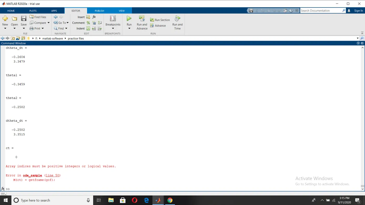
- Counter value should be non-zero.
- We know, the suspension of pendulum is towards negative Y-axis. So that, while calculating y1 length should be negative.
- While creating a video, give names accordingly as shown without any errors because they are in-built MATLAb tools.
- You can also create video in .mp4 format by changing the statement as below.
videofile = VideoWriter('simple_pendulum_motion.mp4')
Errors and rectification:
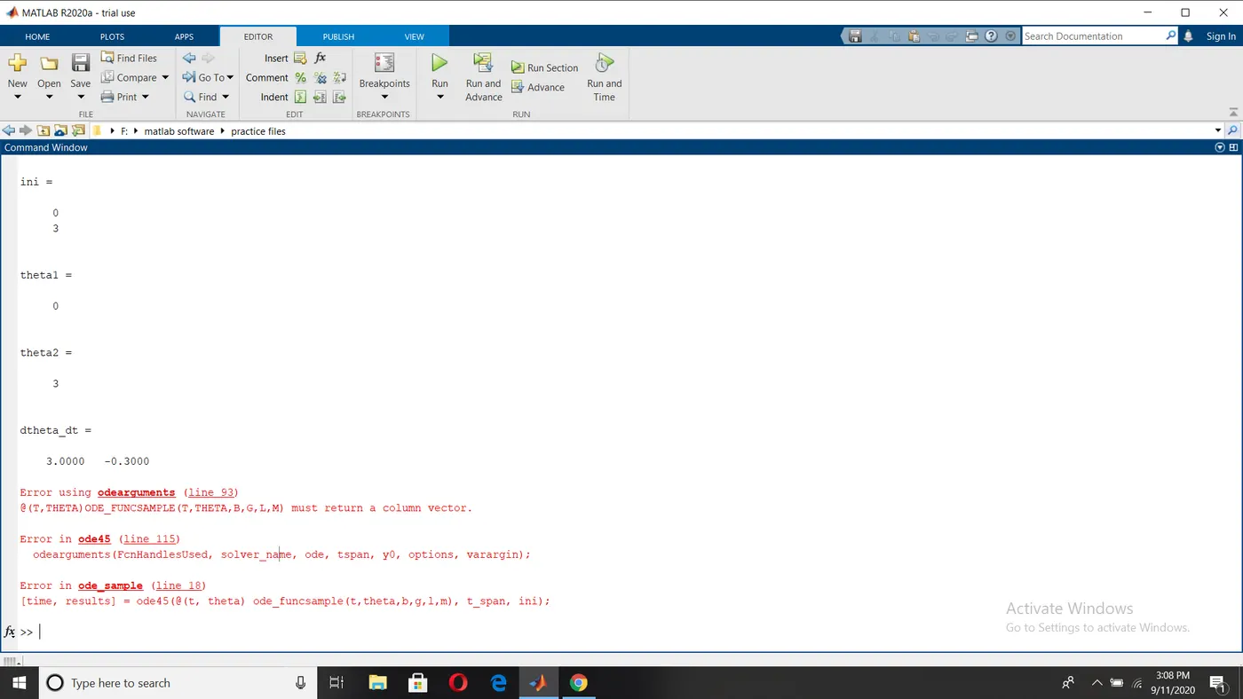
- While solving ODE in main script, use column wise operator only. When ';' is not present in the main script, we get below error.
- When you give counter 'ct' value zero. We get below error.
- When hold on or hold off command is used used correctly. We get error in plots. We also get this type of errors when we terminate or disturb the plots while they are running. We get intermixing of plots or same plots in both figures. So, don't terminate or click anything while plots are creating and hold on and hold off commands should use where there are required. Below is the error when we disturb figures.
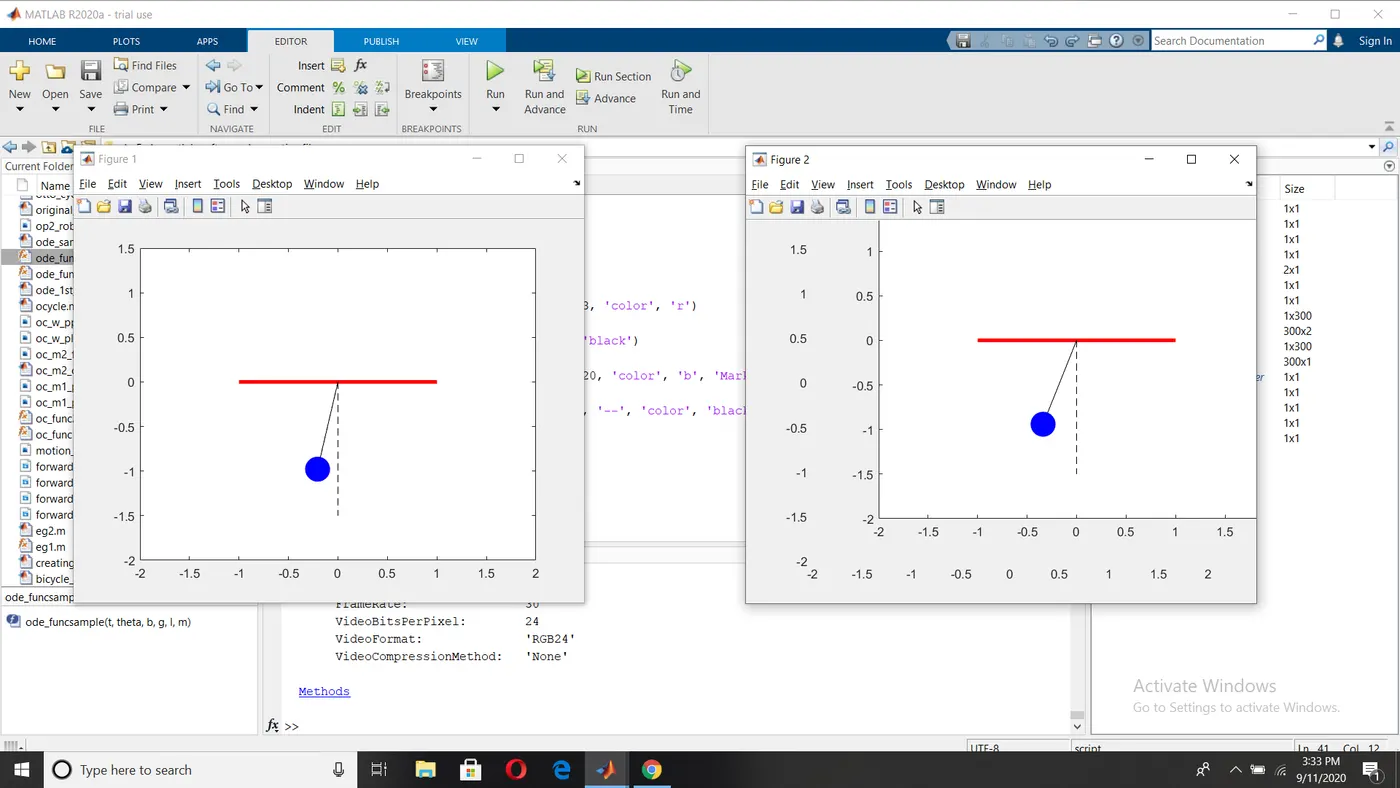
Conclusion: Therefore, the video for the motion of a simple pendulum is created by solve ODE using MATLAB.