Week 3 - Solving second order ODEs

Objective - A program that will simulate the pendulum motion, with given requirements.

Report

1) The complete program used to run the simulation

clear all
close all
clc

% Defining the parameters
% Given
b= 0.05
g=9.81
l=1
m=1

% Defining initial conditions for displacement and velocity
theta_i=[0;5]

% Defining the time points (as mentioned)
time_span=linspace(0,20,500)

% Solving
% Using ode45 command to solve the ode equation
% Calling the function defined in another program
[t,results]=ode45(@(t,theta)ode_function(t,theta,b,g,l,m),time_span,theta_i);

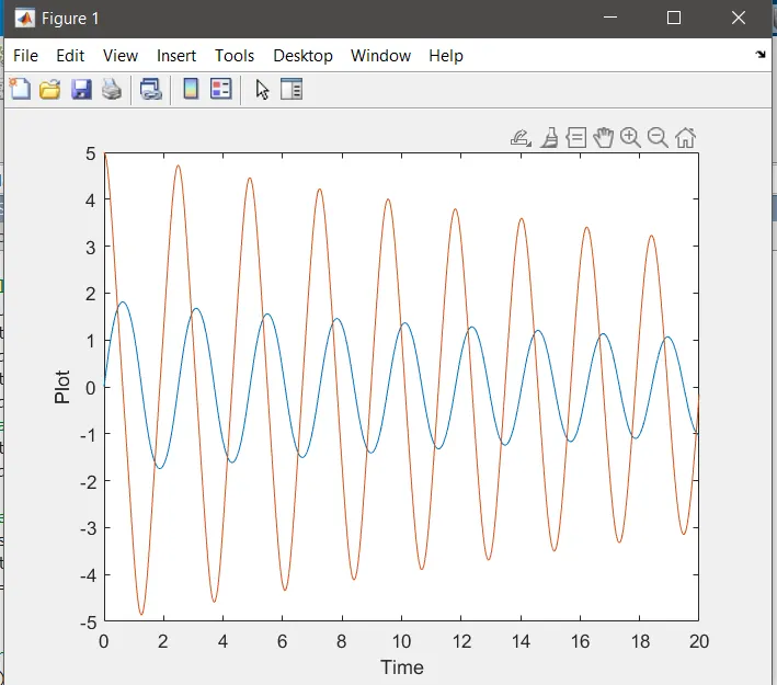
% Plotting the graph displaying displacement and velocity against time
plot(t,results(:,1))
hold on
plot(t,results(:,2))
% Labelling the axes
xlabel('Time')
ylabel('Plot')

% Assigning displacement values to another variable theta2
theta2 = results(:,1);

% Initiating For loop for simulating the movement of varying pendulam in
% accordance with varying displacement values

ct=1
for i = 1:length(theta2);
    
    % Assigning a variable to the varying theta2 values
    theta_x = theta2(i);           
    
    % Stating the starting points
    x0= 0;
    y0= 0;
    
    % Stating the end points of the pendulam 
    x1 = l*sind(theta_x); 
    y1 = -l*cosd(theta_x);
   
    
    % Plotting the pendulum movement
    figure(2)
    plot([-0.5 0.5],[0 0],'color','b',LineWidth=4);
    hold on 
    plot([x0 x1],[y0 y1],'color','r','linewidth',2)
    hold on 
    % Marker command used for displaying the pendulam ball
    plot(x1,y1,'o','markers',15,'markerfacecolor','y')
    hold off
   
    % Defining axis
    axis([-2 2 -2.5 1]);
    M(ct) = getframe(gcf);
    ct = ct+1;
end

% Command to save the animation of the pendulam
movie(M)
videofile = VideoWriter('pendulum.avi','Uncompressed avi');
open(videofile)
writeVideo(videofile,M)
close(videofile)

2) Program used as a function

function [dtheta_dt]= ode_function(t,theta,b,g,l,m)
 
theta1=theta(1)
theta2=theta(2)
dtheta1_dt =theta2;
dtheta2_dt=(-b/m)*theta2-(g/l)*sin(theta1);
dtheta_dt=[dtheta1_dt;dtheta2_dt]
end

Step By Step process

1. Defined the parameters already given as input in the question

2. Defined initial condition for displacement and velocity as displacement starting 0, and velocity mentioned 3 rad/sec

3. Defined the time span as mentioned

4. Created another program to define the function ode_function

5. The function is created to make a 2nd Order Differential equation into two 1st order differential equation

6. We called this function in the main program along with ode45, which is ODE solver command in matlab using time and theta as differential factors of the equation

7.We then plot a graph displaying displacement and velocity as a function of time

8. Taking all the rows in the first column as 1 graph, which is displacement

9. Taking all the rows in the second column as 2nd graph, which is velocity

10. Labelled the axes as Time and plot

11. Now in order to run a simulation

12. Assigned the displacement values to another variable as theta2

13. we intitiate a counter for the for-loop

14. For-loop condition is stated as from 1 to the number of values for displacement

15. Defined the starting and ending points and plotted the graph

16. Used marker command for displaying o as the ball of pendulam

17. saved the animation as a movie command

Result

1) the simulation has been uploaded into youtube, sharing the link below

https://youtu.be/ZK68JXHODno

2) A graph displaying the variation of displacement and velocity against time