Week 5 - Genetic Algorithm

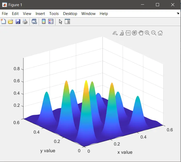
Objective - To write a code in MATLAB to optimise the stalagmite function and find the global maxima of the function.

Report-

Step by Step process

Program 1) A PROGRAM THAT TESTS OUT GENERAL STALAGAMITE AND GENETIC ALGORITHM FUNCTIONS

clear all
close all
clc

% Defining the x and y ranged values using linspace command
x=linspace(0,0.6,150);
y=linspace(0,0.6,150);

% Creating a 2D mesh over the surface of the stalagamite
[xx,yy]=meshgrid(x,y);

% Using for loop to run the loop, and calling of stalagamite function we
% defined in another program
for i=1:length(xx) % range specified
    for j=1:length(yy) % range specified
        input_vector(1)=xx(i,j);
        input_vector(2)=yy(i,j);
        f(i,j)=stalagmite(input_vector);
    end
end

% surf c command to create a 3 dimentional surface plot
surfc(xx,yy,f)
xlabel('x value')
ylabel('y value')
shading interp
% Calling genetic algorithm command with defined syntaxes
[inputs,fval]=ga(@stalagmite,2)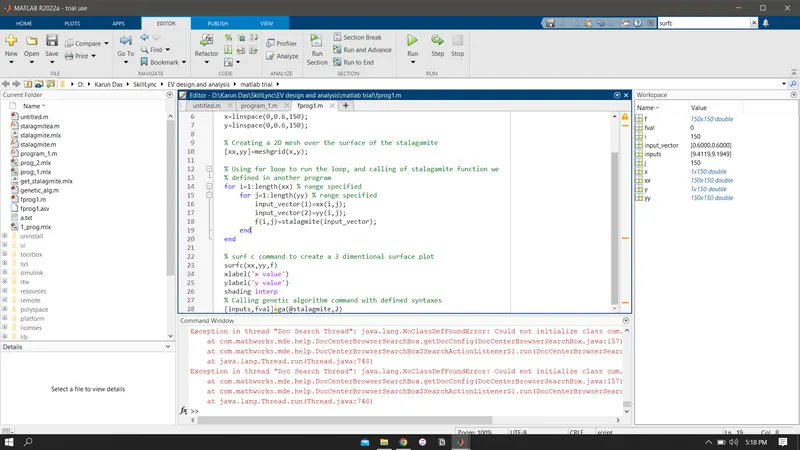

function used-

function [f]=stalagmite(input_vector)

x=input_vector(1);
y=input_vector(2);
f1=(sin(5.1*pi*x+0.5))^6;
f2=(sin(5.1*pi*y+0.5))^6;
f3=exp(-4*log(2)*(x-0.0667)^2/0.64);
f4=exp(-4*log(2)*(y-0.0667)^2/0.64);

f=(f1*f2*f3*f4);
end

Result

Program 2) RUNNING 3 CASES OF OPTIMAL MAXIMA FINDING, GENETIC ALGORITHM COMMAND FUNCTION

clear all
close all
clc

% Defined x and y ranged values using linspaace command
x=linspace(0,0.6,150);
y=linspace(0,0.6,150);

% Adding a 2D mesh grid to the surface
[xx,yy]=meshgrid(x,y);


% Adding for loope and valuating the stalgamitea function
for i=1:length(xx)
    for j=1:length(yy)
        input_vector(1)=xx(i,j);
        input_vector(2)=yy(i,j);
        f(i,j)=stalagmitea(input_vector);
    end
end
surfc(xx,yy,-f)
shading interp
num_cases=50


tic

% Study 1 analysis- Unbound and no additions
for i=1:num_cases
    [inputs,fopt(i)]=ga(@stalagmitea,2);
    xopt(i)=inputs(1);
    yopt(i)=inputs(2);
end

study1_time=toc

% Plotting Study 1 analysis
figure(1)
subplot(2,1,1)
surfc(xx,yy,-f)
hold on
shading interp
plot3(xopt,yopt,-fopt,'marker','o','markersize',5,'markerfacecolor','r')
title('Unbounded inputs')
subplot(2,1,2)
plot(-fopt)
xlabel('Iterations')
ylabel('function minimum')

tic

% Study 2 - Bounded

for i=1:num_cases
 [inputs,fopt(i)]=ga(@stalagmitea,2,[],[],[],[],[0;0],[0.6;0.6]);
    xopt(i)=inputs(1);
    yopt(i)=inputs(2);
end

study2_time=toc

% Plotting of Study 3

figure(2)

subplot(2,1,1)
surfc(xx,yy,-f)
hold on
shading interp
plot3(xopt,yopt,-fopt,'marker','o','markersize',3,'markerfacecolor','g')
title('Bounded inputs')
subplot(2,1,2)
plot(-fopt)
xlabel('Iterations')
ylabel('function minimum')

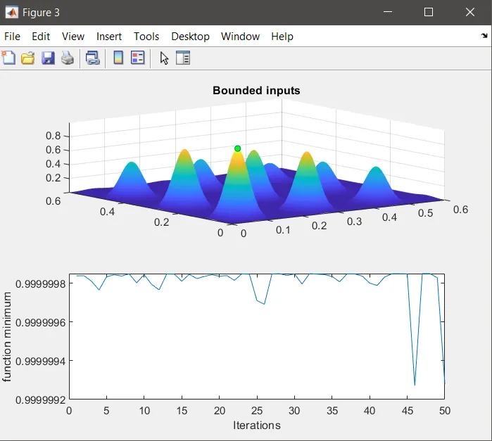
% Study 3- Increasing iteration by increasing the values 
options=optimoptions('ga','populationsize',170)

tic

for i=1:num_cases
 [inputs,fopt(i)]=ga(@stalagmitea,2,[],[],[],[],[0;0],[0.6;0.6],[],[],options);
    xopt(i)=inputs(1);
    yopt(i)=inputs(2);
end

study3_time=toc

% Plotting of Study 3

figure(3)
subplot(2,1,1)
surfc(xx,yy,-f)
hold on
shading interp
plot3(xopt,yopt,-fopt,'marker','o','markersize',5,'markerfacecolor','g')
title('Bounded inputs')
subplot(2,1,2)
plot(-fopt)
xlabel('Iterations')
ylabel('function minimum')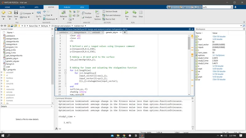

Function used

function [f]=stalagmitea(input_vector)

x=input_vector(1);
y=input_vector(2);
f1=(sin(5.1*pi*x+0.5)).^6;
f2=(sin(5.1*pi*y+0.5)).^6;
f3=exp(-4*log(2).*(x-0.0667).^2/0.64);
f4=exp(-4*log(2).*(y-0.0667).^2/0.64);

f=-(f1.*f2.*f3.*f4);
end

Result

Figure 1

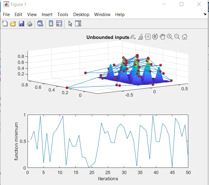
Figure 2

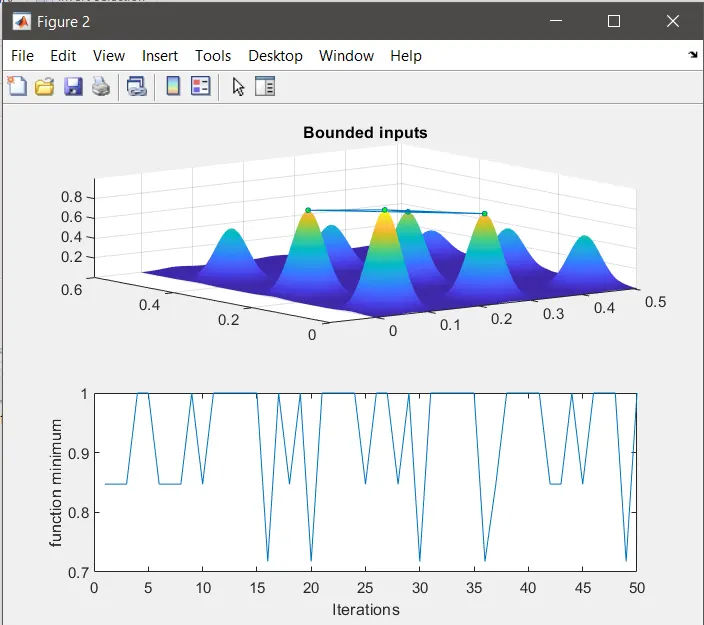
Figure 3

Definition

Genetic algorithm - ga - The algorithm repeatedly modifies a population of individual solutions, at each step. We can apply the genetic algorithm to solve problems that are not well suited for standard optimization algorithms, including problems in which the objective function is discontinuous, nondifferentiable, stochastic, or highly nonlinear.