Week 3: Flow over a backward facing step
Flow over a backward-facing step.
Abstract:
The backward-facing step is an illustration model for separation flows which are seen widely in aerodynamics flows, engine flows, condensers, vehicles, heat transfer systems, and flow around buildings, etc. The flow separation after a simple stage will introduce separation bubble formation, evolution, and re-attachment process. Here in this project, the materials taken, simulation parameters involving solver, solver parameters, initial and boundary conditions, physical models, and three different base grids were taken in Converge Studio for a backward-facing step case and were solved. Pressure and velocity contours, plots of average velocity, mass flow rate, and total pressure were shown. Discussion on why the separation of flow is taking place is done.
Objective:
1. Importing backward-facing step geometry and setup the case with appropriate material properties, boundary conditions, and different base grid sizes.
2. Run the simulation using the CYGWIN terminal. Plot mass flow rate, average velocity, and pressure plots using Converge software line plotting. Obtain velocity and pressure contours using ParaView software.
3. Interpret the results for different base grid sizes and follow them with a discussion.
Procedure:
1. Upload the given .stl file to Converge studio and change the scale to meters if the given geometry is not in meters by going to the scale option under transform.
2. Transform the normal of each triangle to the inside of the wall since internal flow is happening.
3. Boundary condition – Inlet, Front, Back, Top and Bottom, and Outlet are given.
Case-setup:
1. Application: Time-based.
2. Materials:
i) Gas simulation: Air.
ii) Global Transport Properties: Default.
iii) Species: Add O2 and N2.
3. Simulation parameters:
i) Run parameters:
a. Solver: Steady-state solver.
b. Simulation mode: Full hydrodynamic.
c. Gas flow solver: Compressible.
d. Steady-state monitor: on.
ii) Simulation time parameters:
a. Start time: 0.
b. End time: 15000.
c. Initial time-step: 1e-6.
d. Minimum time-step: 1e-6.
e. Maximum time-step: 1.
f. Maximum convection CFL limit: 1.
iii)Solver parameters:
a. Navier-Stokes solver type: Density-based.
b. Equations: Change preconditioner in Pressure to none.
c. Steady-state solver control: Maximum convection CFL limit: 0.8.
iv) Boundary conditions:
a. Inlet: Inflow, Total pressure: 110325 Pa, Initial temperature: 300K and add Species: Air.
b. Front: Two_D.
c. Back: Two_D.
d. Top and Bottom: Wall, Surface movement: Law of wall, Temperature boundary condition: Zero normal gradient and Turbulent kinetic energy boundary condition: Zero normal gradient.
e. Outlet: Pressure: 101325, Temperature backflow: 300K and add Species: Air.
v)Initial conditions and events:
a. Species: Add Air and change the mass fraction of N2 to 0.23 and O2 to 0.77 so that we can see the changes in post-processing and even if the composition is different from the actual mole fractions of air, converge still accepts inputs and gives results according to input.
b. Add region and name it: volumetric region user-defined.
vi) Physical models:
a. Turbulence modeling [RANS_K_EPS_RNG].
vii) Grid control:
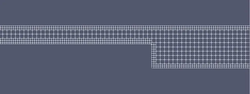
a. Base grid:
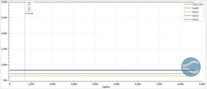
Case-1: dx: 2e-3, dy: 2e-3 and dz: 2e-3.
Case-1: dx: 1.5e-3, dy: 1.5e-3 and dz: 1.5e-3.
Case-1: dx: 1e-3, dy: 1e-3 and dz: 1e-3.
b. Add Fixed embedding. Entity type: Boundary, Boundary ID: Top and Bottom, Mode: Permanent, and Scale: 1. Embedding is useful if you are looking to refine the near-wall mesh to capture the boundary layer accurately.
viii) Output/Post-processing:
a. Select parameters needed and select N2 and O2 in mole fraction under species.
b. Output files: Writing time intervals: Time interval for writing 3D output data files: 150 and Time interval for writing restarting output: 1000.
Results:
Case-1:
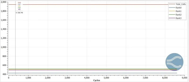
Grid size: dx: 2e-3, dy: 2e-3 and dz: 2e-3.
Mesh:
Cell count:
Velocity contour:
Pressure contour:
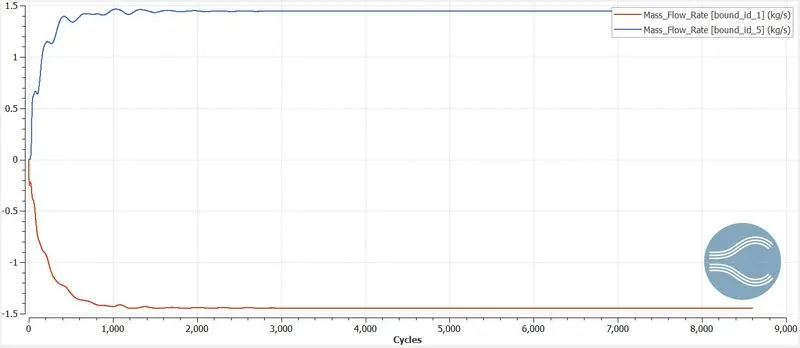
Mass flow rate plot:
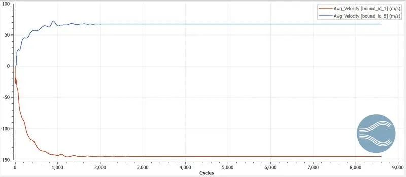
Average velocity plot:
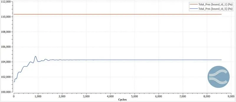
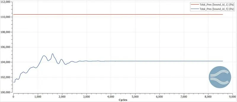
Total pressure plot:
Case-2:
Grid size: dx: 1.5e-3, dy: 1.5e-3 and dz: 1.5e-3.
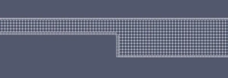
Mesh:
Cell count:
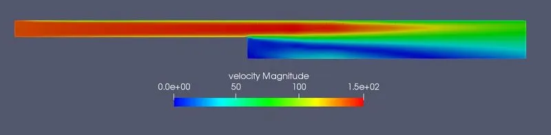
Velocity contour:
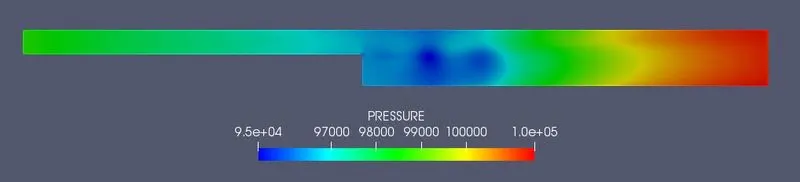
Pressure contour:
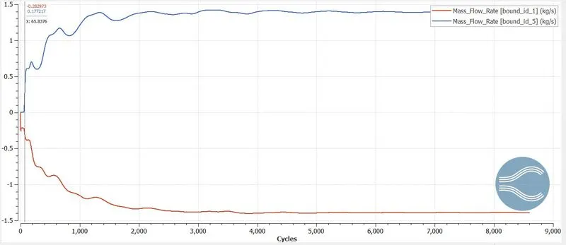
Mass flow rate plot:
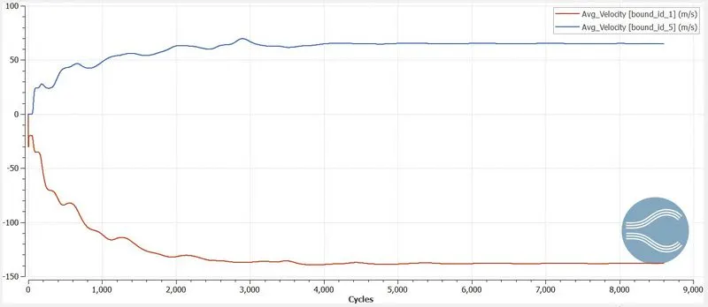
Average velocity plot:
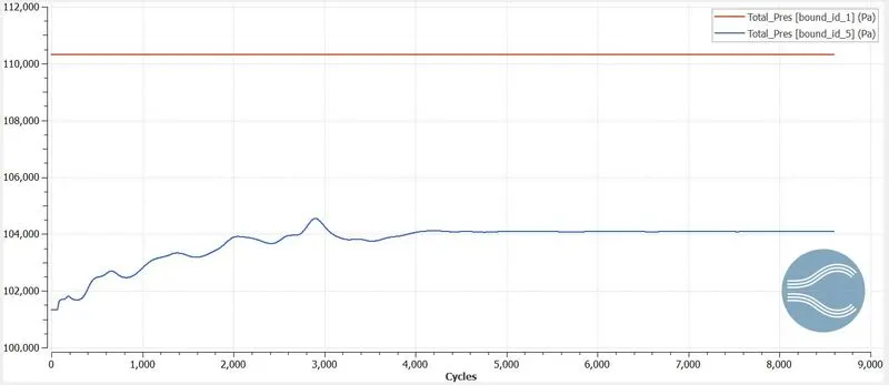
Total pressure plot:
Case-3:
Grid size: dx: 1e-3, dy: 1e-3 and dz: 1e-3.
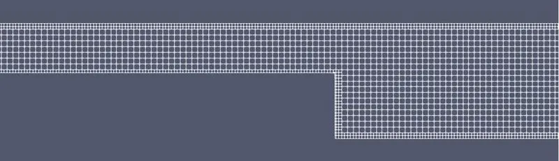
Mesh:
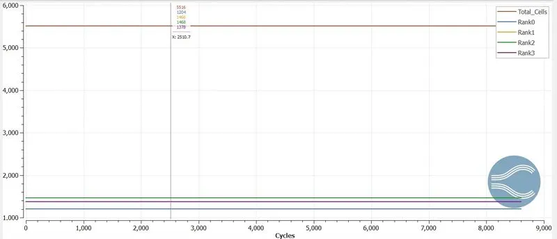
Cell count:
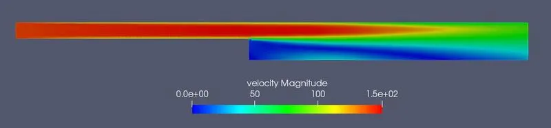
Velocity contour:
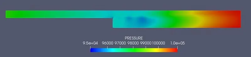
Pressure contour:
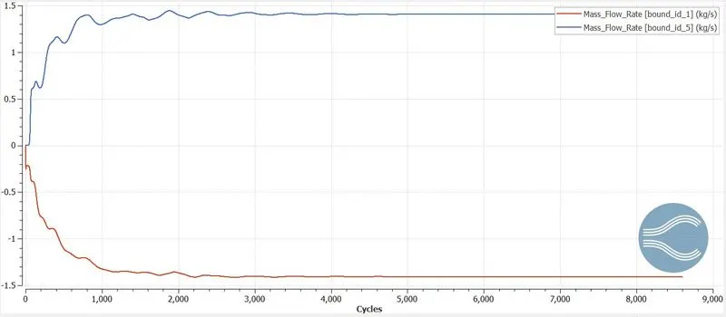
Mass flow rate plot:
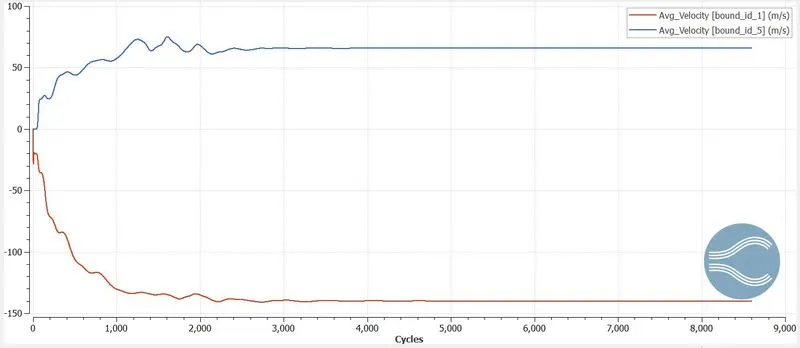
Average velocity plot:
Total pressure plot:
Discussions/Conclusions:
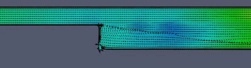
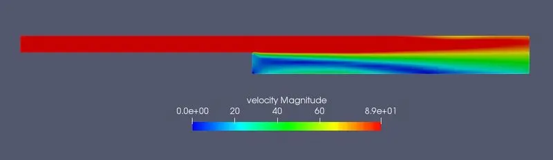
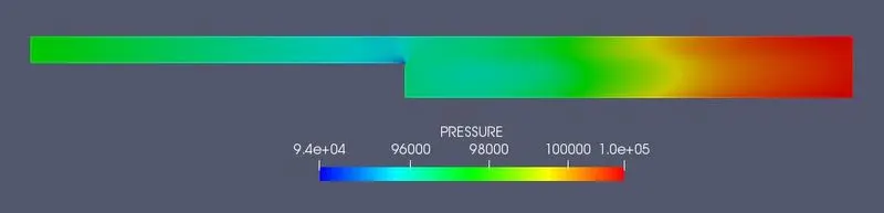
2-D simulation of a backward facing step flow having an RNG K-E model and pressure difference for the momentum of flow is done and velocity and pressure contours along with different plots are shown.
From the above image, we can observe the general characteristics of the flow begins where the upstream boundary layer develops and the pressure gradient is developed into the thin shear layer. Flow separation or boundary layer separation is the disengagement of a boundary layer from a surface into a wake. In the flow that is slowing down, with pressure increasing, after passing the thickest part of a streamline body or passing through a widening passage, separation occurs. Flowing against an increasing pressure is known as flowing in an adverse pressure gradient. The boundary layer separates when it has traveled far enough in an adverse pressure gradient that the speed of the boundary layer relative to the surface has stopped and reversed direction. The flow becomes detached from the surface and instead takes the forms of eddies and vortices. When the Pressure tends to increase after the flow separation point, potential energy develops at the local boundary layer and this causes the reduce the kinetic energy and therefore the velocity reduces. The fluid exerts constant pressure on the surface once it has separated instead of a continually increasing pressure if still attached. The reattachment length is the distance between the step and the reattachment point. After both recirculations of flow occur, it flows towards the outflow direction in order to discharge from the channel.
Flow separation can be reduced by modifying the geometry of the object induced to flows where the boundary layer is continuous and separation occurs at a minimum amount. Flow separation tends to reduce lift and increase static pressure, which can lead to stall for aerodynamic structures. Flow separation creates a wake region at the flow end which causes a recirculation region due to the adverse pressure gradient, creating turbulence and the formation of eddies.