Week 7: Shock tube simulation project
Shock tube simulation project
Abstract:
The report contains a detailed description of the Shock tube Simulation problem using converge CFD software, solving it using CYGWIN, and post-processing the result using ParaView. This Case Study contains a rectangular duct that has two sections along with a diaphragm in between. A high-pressure reservoir is connected to the low-pressure section.
Shock Tube:
A shock tube is a device for studying shock waves. Before starting an experiment, a diaphragm inside the tube blocks any flow. We can increase the pressure on one side, such as with a compressor, and then start the flow by rupturing the diaphragm. The gas expands down the other half of the tube. A high-temperature supersonic gas flow is initiated in a shock tube as a result of rupture of a diaphragm separating two gases in high-pressure and low-pressure chambers. An unsteady rarefaction wave passes into the "driver" gas in the high-pressure chamber with a velocity of a few kilometers per second. This results in the drivers' gas flowing into the low-pressure gas, pushing the gas in the low-pressure chamber ahead of it. The shock wave propagates in the low-pressure chamber ahead of this flow of the studied gas. The velocity of the driven gas flow is equal to that of the driver gas flow.
Objective:
1. The major objective of this project was to set up Transient Simulation in a Shock Tube using Converge CFD. A shock tube that has a diaphragm in between and the tube is one side filled with high-pressure Nitrogen where the other side is filled with low-pressure Oxygen.
2. Plot the pressure and temperature history in the entire domain - Explain the result.
3. Plot the cell count as a function of time - Explain the result.
Geometry:
Import the geometry into the Converge studio and clean up the geometry by using some tools which are available in the converge.
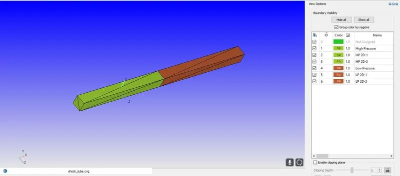
Enable the vectors on the geometry to make sure that all the normals should be facing inside the fluid domain The below figure shows the vectors outside the domain convert them into inside where the fluid is going. Now check for the errors in the geometry by opening the diagnosis dock and then find if no errors are there means we can proceed to the case setup.
Case setup for Simulation:
• Application Type-Time Based
• The flow is the general flow that contains the air as a Material.
• Air contains a Species mixture of O2 and N2 which will flow through the required geometry.
• Global Transport Parameters the Prandtl number is 0.9 and the Schmidt number is 0.78.
Simulation Parameters:
• In the Run Parameter: Solver we used is Transient state and the simulation mode Full hydrodynamic in the mic state we enable the Solver Momentum, Solve Species.
• In Simulation time Parameters we set the values for start time as O Seconds and end time as 0.003 Seconds and the initial and Minimum time setup for le-9 and Maximum time setup is 1 sec and the remaining values are put to default.
• In the Solver Parameters, the Navier stock equation should be a pressure-based solver, and the remaining should be the default.
Initialization and Boundary Conditions:
• In the initialization region we have to create the two regions and initialized them with the values.
• The name of the Region is High-Pressure Region and the values assigned for the temperature and pressure are 300k and 600000 Pascal and add the species N2 with the mole fraction of 1.
• The name of the other Region is Low-Pressure Region and the values assigned for the temperature and pressure is 300k and 101325 Pascal and add species O2 with the mole fraction of 1.
Events:
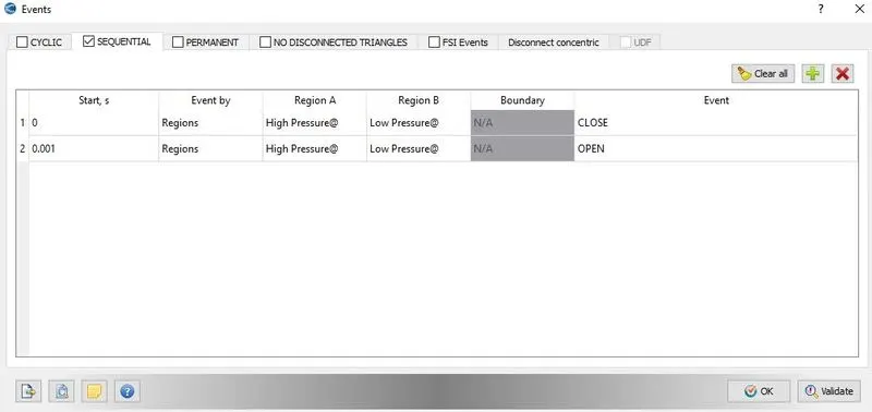
CONVERGE uses events to active or deactivate the disconnect triangles, which control when and where flow between regions is allowed. An OPEN event deactivates the disconnect triangles and thus allows flow between the specified regions. A CLOSE event activates the disconnect triangles and thus prohibits flow between the specified regions. When disconnect triangles are activated, they act as a SYMMETRY boundary condition.
The Events must be CYCLIC, SEQUENTIAL, PERMANENT, or NO_DIS_TRIANGLES.
In this, we used the Event as Sequential.
• At O seconds the diaphragm between the High-Pressure Region and Low-Pressure Region is closed.
• After 1 millisecond the diaphragm between the High-Pressure Region and Low-Pressure Region is open.
High-Pressure Region Boundary Conditions:
• For the high-pressure region the boundary type should be wall.
•Velocity Boundary Condition should be the Slip Condition.
• Temperature Boundary Conditions should be the Zero Normal Gradient.
Low-Pressure Region Boundary Conditions:
• For the Low-pressure region the boundary type should be wall.
• Velocity Boundary Condition should be the Slip Condition.
•Temperature Boundary Conditions should be the Zero Normal Gradient.
Physical Models:
• In the physical models, the Turbulence Modelling and the solver should be selected as RNG K-e and put the remaining values as a default.
Grid Control:
• Element size dx-dy-dz-0.003 m.
Adaptive mesh refinement (AMR):
In numerical analysis, adaptive mesh refinement (AMR) is a method of adapting the accuracy of a solution within certain sensitive or turbulent regions of simulation. dynamically and during the time the solution is being calculated. When solutions are calculated numerically, they are often limited to pre-determined quantified grids as in the Cartesian plane which constitutes the computational grid, or 'mesh. However, many problems in the numerical analysis do not require a uniform precision in the numerical grids used for graph plotting or computational simulation and would be better suited if specific areas of graphs that needed precision could be refined in quantification only in the regions requiring the added precision. Adaptive mesh refinement provides such a dynamic programming environment for adapting the precision of the numerical computation based on the requirements of a computation problem in specific areas of multi-dimensional graphs which need precision while leaving the other regions of the multi-dimensional graphs at lower levels of precision and resolution.
In our case, we need more refinement of mesh at the region of shock and the remaining should be the normal grid size mesh.
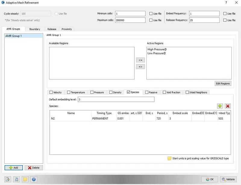
In Converge we have the different methods which are used for the Adaptive Mesh Refinement Right now we are using the species-based method with the 3 embedded level. Thus, the converge helps the curvature of temperature property provided in AMR and starts refining the mesh for the temperature curvature.
• In the Grid control enable the Adaptive Mesh Refinement
• In Adaptive Mesh Refinement the High Pressure_region and
• Low-pressure region is changed from the Available region to the Active Region.
• Then Go to Species
• Enter the number of Embedded level=3
• In the species window enter the details as per the below figure:
Output and Post Processing:
• Post variable Selection and Output files are the default values.
• In the output files we have given a time interval to write the 3D output data=0.00003 Seconds, thus the outputs of the simulation files be stored after 0.00003 seconds.
Post-Processing:
Post-processing of the results for the case has been done using the converge studio and ParaView. Post-processing is actually used in order to get the desired Output by running the simulation.
Results:
Mesh:

Moving Mesh:

Pressure Plot and Contour:
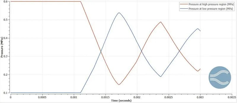
As the pressure difference between the two regions is 5 bar. As the mixing occurs the pressure difference occurs in both regions. As the high-pressure gas starts mixing with the low-pressure gas, thus it leads to the formation of shock waves due to the difference in the pressure. These shock waves travel to and fro in the domain due to the reflection from the walls. The pressure of N2 gets dropped due to the expansion and the pressure for the O2 gets increases due to the Compression of gas. When the wave gets back to its original position the pressure again increases and the pressure in the low region decreases we can clearly observe this change in the graph for maxima and minima graphs. This process continues till it reaches the simulation time.
Contour: https://youtu.be/_2g_1TcPVpc
From the above animation, we can see that the waves are traveling from higher pressure region to lower pressure region and when it reaches the dead-end it reflects back and travels in the opposite direction and the process repeats.
Temperature Plot and Contour:
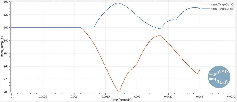
From the graph, in the higher pressure region, the temperature is constant at the initial stage. After 1 millisecond the temperature declined a lot from 300 k to200 k due to the pressure decrease in the domain. At the same time, the temperature in the lower region increases due to the pressure increase. We can see the fluctuations in the graph due to the shock wave as it moves front and back in the domain. When it moves backward the temperature in the high region starts increasing and decreases in the low region. Simultaneously it happing as the flow waves are moving forward and backward.
Contour: https://youtu.be/Yex94G2InlI
Velocity Contour:
Contour: https://youtu.be/BTQzTP0E-68
Total Cell count:
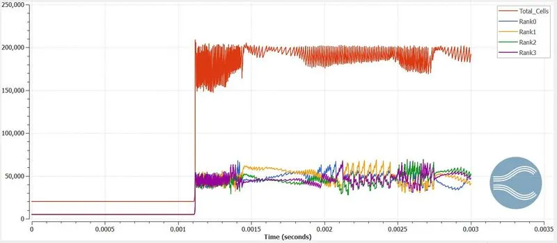
As we have specified the Adaptive meshing options under the species properties, we can see that the meshing gets refined at the areas where the Species mass fraction differs. For 0.001 seconds both the species in the two regions stay undisturbed as the path between the regions is closed. As time increases the path gets opened and the flow happens from the high-pressure region to the low-pressure region. Thus after 0.001 seconds, the flow takes place, and the mass fraction of the species changes which in turn refines the meshing at the areas where the flow occurs.
Conclusion:
High-Pressure N2 gas compresses the low-pressure 02 then after some compression a recirculation takes place and the low-pressure gas passes the N2. From this problem, we can understand the compressibility of gas and study the flow. Due to adaptive mesh refinement, the cell count is varying all the time when the expansion and contraction are taking place inside the shock tube. From the pressure plot, it can be concluded that after some time both the species will have common pressure as one pressure is increasing and the other is decreasing wrt time. The temperatures first fluctuate then will attend the equilibrium position after some time. Learned the purpose of concept called "Events".