Week 4.2: Project - Transient simulation of flow over a throttle body
Transient simulation of flow over a throttle body:
Abstract:
A throttle body controls airflow and plays a major role in the performance and efficiency of a spark-ignition engine. Controlling airflow into the engine is a crucial factor in controlling the engine’s air/fuel ratio. Throttle bodies usually use butterfly valves. These valves consist of a casing with a large hole in the center, which is filled with a steel plate called a butterfly, or throttle plate. The throttle shaft is a rod that passes through the housing and is connected to the throttle cable on the outside and the throttle plate on the inside. When the throttle shaft turns, it rotates the throttle plate, allowing air to go around it and into the engine. The throttle plate also acts as a restriction to the intake air stream, causing loss of flow energy in the intake air. In this project, transient simulation for airflow in an elbow containing a throttle has been carried out using Converge CFD to understand the behavior of airflow inside and a comparative study of pressure and velocity variations across the valve has been done.
Objective:
1. The objective of the project is to setup and simulate transient airflow in an elbow with a throttle using Converge CFD and CYGWIN Terminal.
2. Show pressure and velocity contours inside the elbow with throttle present using ParaView software and plot mass flow rate, average velocity, total pressure, and total cell count graphs using Converge software line plotting.
3. Show the calculations on how end time is calculated.
Work Flow involved:
1. Pre-processing (preparing surface geometry, giving rotating center and rotating normal for throttle, meshing, and configuring the input and data files).
2. Running the simulation.
3. Post-processing (showing of different contours and plots involved).
1. Pre-processing:
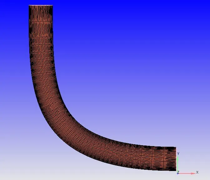
1. Upload the given .stl file to Converge studio and change the scale to meters if the given geometry is not in meters by going to the scale option under transform.
2. Transform the normal of each triangle to the inside of the wall since internal flow is happening.
3. Boundary condition – Elbow wall, Throttle, Inlet and Outlet are given.
Geometry:
Case-setup:
1. Application: Time-based.
2. Materials:
i) Gas simulation: Air.
ii) Global Transport Properties: Default.
iii) Species: Add O2 and N2.
3. Simulation parameters:
i) Run parameters:
a. Solver: Transient.
b. Temporal type: Time-based simulation
c. Simulation mode: Full hydrodynamic.
d. Gas flow solver: Compressible.
ii) Simulation time parameters:
a. Start time: 0.
b. End time:
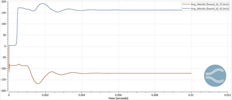
From my previous project: https://skill-lync.com/projects/week-4-1-project-steady-state-simulation-of-flow-over-a-throttle-body-24, from the average velocity graph, at the inlet velocity is nearly 200 m/s due to the pressure difference. And the maximum length for the elbow cannot be greater than 0.2m which is measured in converge studio.
So, Flow-through time = Characteristic length/Average velocity.
Flow-through time = 0.2/200 = 0.001.
Simulating the flow till roughly 10 times the flow-through time 1e-3 10 = 0.01 seconds.
Rounding off the end time to 10 milliseconds.
c. Initial time-step: 1e-9.
d. Minimum time-step: 1e-9.
e. Maximum time-step: 1.
f. Maximum convection CFL limit: 1.
iii)Solver parameters:
a. Navier-Stokes solver type: Density-based.
b. Equations: Change preconditioner in Pressure to none.
iv) Boundary conditions:
a. Elbow wall: Wall, Surface movement: Law of wall, Temperature boundary condition: Zero normal gradient and Turbulent kinetic energy boundary condition: Zero normal gradient.
b. Throttle: Wall, Wall rotating type: Rotating, Surface movement: Moving, and Turbulent kinetic energy boundary condition: Zero normal gradient.
We need to find the Rotate center and Rotate about and can be done using the following operations:
Geometry > Measure > Direction > Direction options - Arc normal > vertex as an entity selection-By Any> using cursor pick option>Selecting the three vertices on the arc as shown in below image> Apply.
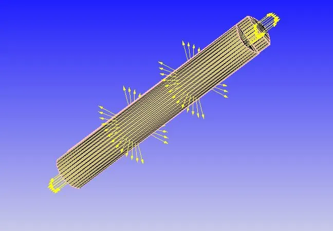
The normal arrows show the direction it should rotate about.
The following are the Rotate center and Rotate about values.
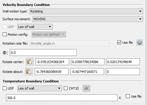
For Rotation rate file: Use file.
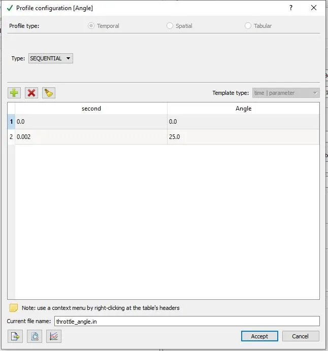
From 0 to 2 ms, the rotation angle will change to 25 degrees and stay till the end of the flow.
c. Inlet: Inflow, Total pressure: 150000.0 Pa, Initial temperature: 300K and add Species: Air.
d. Outlet: Pressure: 100000.0, Temperature backflow: 300K and add Species: Air.
v)Initial conditions and events:
a. Species: Add Air and change the mass fraction of N2 to 0.23 and O2 to 0.77 so that we can see the changes in post-processing and even if the composition is different from the actual mole fractions of air, converge still accepts inputs and gives results according to input.
b. Add region and name it: volumetric region user-defined.
vi) Physical models:
a. Turbulence modeling [RANS_K_EPS_RNG].
vii) Grid control:
a. Base grid:
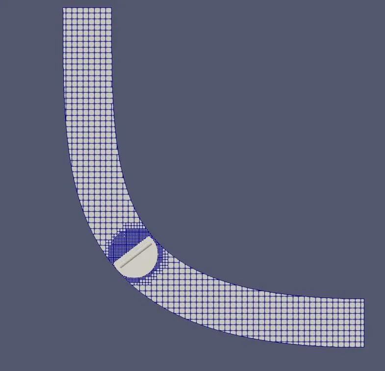
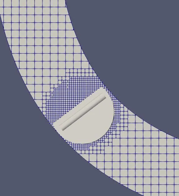
Converge CFD uses a cut-cell cartesian method. Mesh refinement can be performed at locations where the flow properties need to be captured accurately. A method called "Fixed Embedding" is deployed in this case with the region near the throttle body being the region of interest.
The scaling factor of 2 has been used with 2 layers of fixed embedding.
dx: 2e-3, dy: 2e-3 and dz: 2e-3.
b. Add Fixed embedding. Entity type: Boundary, Boundary ID: Throttle, Mode: Permanent, Scale: 2, and Embed Layers: 2. Embedding is useful if you are looking to refine the near-wall mesh to capture the boundary layer accurately. The scaling factor of 2 has been used with 2 layers of fixed embedding. The base grid used in this simulation is 2e-3 in x, y, and z-direction. This means that after scaling has been applied for the mesh near the throttle valve region, the mesh will be of value 4e-3. The refined mesh near the throttle valve and the base mesh can be seen in the figures down below
viii) Output/Post-processing:
a. Select parameters needed and select N2 and O2 in mole fraction under species.
b. Output files: Writing time intervals: Time interval for writing 3D output data files: 0.001 and Time interval for writing text output: 1e-6.
2. Running the simulation:
After this, we need to export the data. To do that, 'File' > 'Export' > 'Export input files'.
Open Cygwin and navigate to the folder in which the input files are exported and run the command as 'mpiexec.exe -n 4 converge.exe restricted' and then press enter. The simulation will run and in the end, if it shows 'normal termination', the simulation has ended successfully.
3. Post-processing and Results:
All the post-processing of results is done in ParaView software after extracting the output file from converge.
Mass flow rate:
For a steady-state simulation, it is important to check if convergence has been attained. To do so, it is a good idea to analyze mass flow rate plots for inlet and outlet sections. The mass flow rate plot can be seen in the below figure.
Mass_Flow_Rate [bound_id_3]: Inlet.
Mass_Flow_Rate [bound_id_4]: Outlet.
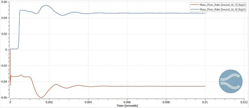
The above plot shows that the mass flow rate initially takes a little turbulence and finally converges as expected. From the above figure, convergence for both the inlet and the outlet section occurs at approximately 0.045 kg/s mass flow rate.
Total cell count:
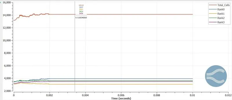
The total cell count is 14114 and is distributed between 4 processors.
Throttle movement:
The link for throttle movement: https://youtu.be/tCjCtWJPwPU
We can see the throttle movement by an angle 25 degrees.
Velocity Contours:
The link for velocity contour front side: https://youtu.be/wUN8ZCPKnEI
The link for velocity contour backside: https://youtu.be/JYU6YZylznk
The link for velocity contour: https://youtu.be/zanmqatRLOw
The velocity vectors for the front and backside are shown below:
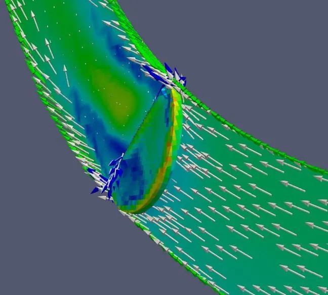
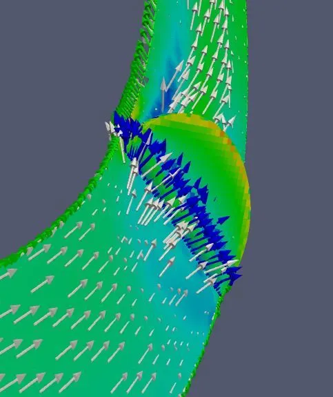
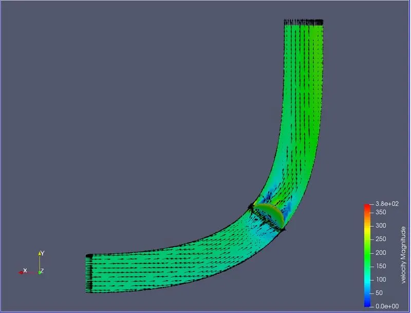
The velocity contours at the end of the simulation are shown below:
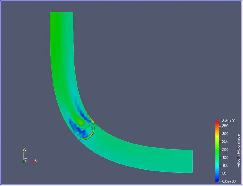
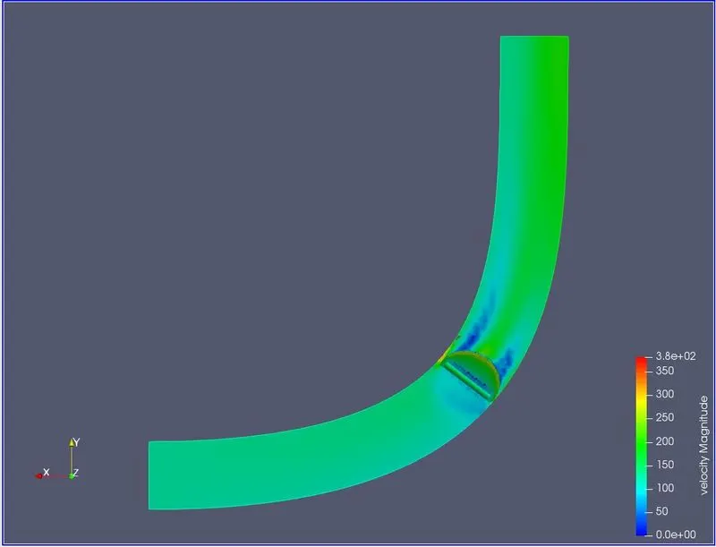
The maximum velocity is achieved when the throttle is open, ie it is aligned/ parallel to the flow direction.
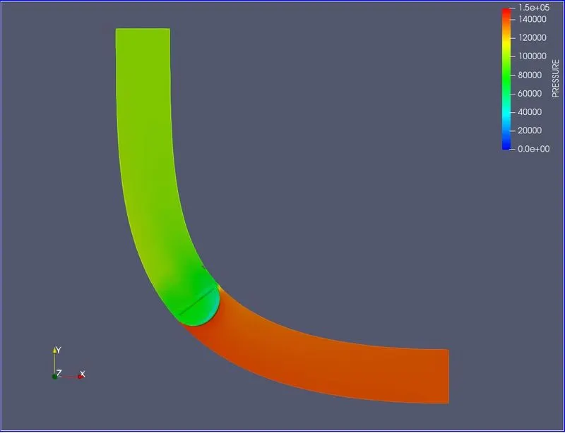
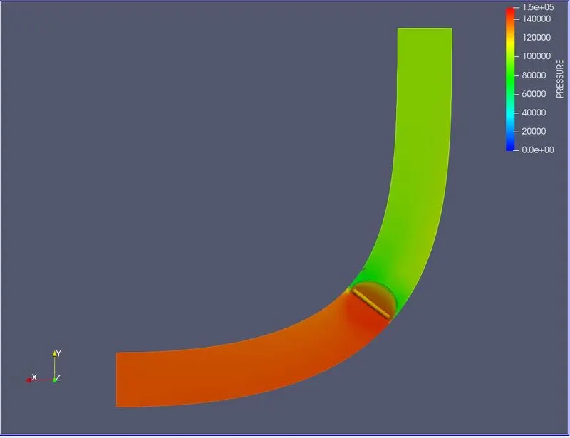
Pressure contours:
The link for pressure contour front side: https://youtu.be/sGy5Bd8Ieng
The link for pressure contour backside: https://youtu.be/tpC_IsYnJ18
The link for pressure contour: https://youtu.be/5BqMIgbWe2c
Pressure contours at the end of simulation for front and backside are shown below:
Average velocity plot:
Total pressure plot:
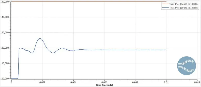
Total_Pres [bound_id_3]: Pressure at the inlet: 150000 pa.
Total_Pres [bound_id_4]: Pressure at the outlet can be seen varying and then settling down below 120000 pa.
Conclusions:
Transient simulation analysis of an elbow containing a throttle body is done. Velocity and pressure contours along with plots of mass flow rate, average velocity, total pressure, and cell count are shown. Through contour plots for velocity and pressure, it is observed that the movement of the throttle impacts the velocity and pressure in the region rear to the throttle valve. Also, the movement of the throttle has an impact on the cell count until 2 milliseconds.