Week 6: Conjugate Heat Transfer Simulation
Conjugate Heat Transfer Simulation:
Aim: In this project, we simulate the flow of air through an aluminium pipe that is heated from the outside. We observe the conjugate heat transfer and derive appropriate results that include plots and contours for temperature, velocity, etc We also understand the concept of super-cycling. We also need to perform a grid dependence test for different grid sizes to show that the temperature at the outlet converges to a particular value.
Given: Reynolds number = 7000 to calculate inlet velocity which is at 300k.
Conjugate Heat Transfer:
Whenever heat transfer occurs between solid and fluid regions or vice-versa by exchanging their thermal properties at their interface and to simulate this case conjugate heat transfer analysis is used. Conjugate heat transfer (CHT) describes processes that involve variations of temperature within solids and fluids due to thermal interaction between the solids and fluids. In solids, conduction often dominates whereas, in fluids, convection usually dominates.
It helps us to simulate & understand thermal systems like heat sinks, electronics cooling, exhaust port of the vehicle, HVAC, ICE, etc.
Concept of Super-cycling:
CONVERGE Studio uses the Super-cycling method in the case of conjugate heat transfer problems with solid and liquid regions. The integral problem here is that both solvers cannot run at the same speed since solving in the fluid domain is much faster due to the time scale difference for heat transfer in liquids as compared to solids. Problems are caused during the solution given that the solid side solver would not have reached a steady-state/convergence in the time the liquid solver does. This is the juncture where the concept of super-cycling can be used.
Steps of Super-cycling:
Converge solves the fluid and solid together with the transient solver and during this, it stores instantaneous heat transfer coefficients and temperature on the interface during this process.
It freezes the fluid solver and time-averages the heat transfer coefficients and temperature and applies them as boundary conditions at the interface.
Then it solves the solid temperature until it reaches a steady-state.
It updates the solid temperature and unfreezes the fluid solver.
This process repeats until the solid temperature converges.
Conclusion: The basic idea of super cycling is that the solver for the fluid domain is paused until the solver for the solid domain converges.
Output Y+:
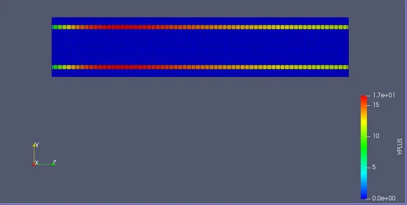
Wall function are useful in telling the solver how to approach the solution near a wall. These are used to predict near-wall results accurately even at a coarse grid. The Y + value is a non-dimensional term that can be used to understand how coarse grid is fine, this can then be used to determine if wall function needs to be used or not.
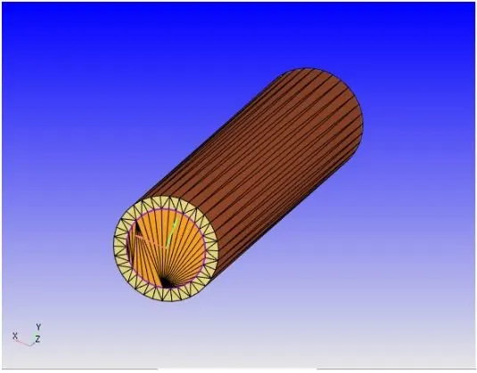
Geometry:
Case-setup:
1. Application: Time-based.
2. Materials:
i) Gas simulation: Air.
ii) Global Transport Properties: Default.
iii) Species: Add O2 and N2.
iv) Solid simulation: Aluminium.
3. Simulation parameters:
i) Run parameters:
a. Solver: Transient.
b. Temporal type: Time-based simulation
c. Simulation mode: Full hydrodynamic.
d. Gas flow solver: Compressible.
ii) Simulation time parameters:
a. Start time: 0.
b. End time: 0.5 s.
c. Initial time-step: 1e-9.
d. Minimum time-step: 1e-9.
e. Maximum time-step: 1.
f. Maximum convection CFL limit: 1.
iii)Solver parameters:
a. Navier-Stokes solver type: Density-based.
b. Equations: Change preconditioner in Pressure to none.
iv) Regions and Initialization:
(0) Fluid region: Temperature- 300 K and Pressure- 101325 Pa
(1) Solid region: Temperature: 300 K.
v) Boundary conditions:
a. Solid outer wall: Wall, Surface movement: Fixed, Slip, Temperature boundary condition: Heat flux = -10000 W/m^2.
b. Solid side: Surface movement: Fixed, Slip, Temperature boundary condition: Zero normal gradient.
c. Outlet: Outflow, Pressure Value set to 101325 Pa at the outlet.
d. Inlet: Inflow, In the problem, it is given that the inlet Reynolds number should be 7000. The value of the inlet velocity is computed to be 3.661 m/s.
Interface. The normals on the interface point towards the fluid region and this is referred to as the forward side. The opposite direction points towards the solid direction referred to as reverse direction.
Velocity and Temperature boundary conditions in forward region set to Law of the Wall.
In Reverse region Velocity and temperature set to slip and specified value respectively.
vi) Physical models:
a. Turbulence modeling [RANS_K_EPS_RNG].
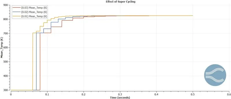
vii) Supercycling was enabled in order to reduce the computational time required for CHT analysis. A monitor point was created at the outlet. Time length was initially set to 0.05 for base grids- 0.004, 0.003, and 0.002. Then reduced to 0.03.0.02 and 0.01 for a base grid of 0.003 to study the super cycling effect.
In order to execute the simulation, the directory in which these input files were stored was accessed in Cygwin and the following command was typed "mpiexec.exe -n 4 converge.exe" After the Simulation was executed, the results were converted into a form that would be compatible with Paraview. This was done using the post convert.exe command.
Results:
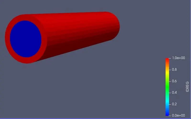
Differentiating solid (red) and fluid (blue) regions.
Case-1 (Base grid- 0.004 with super cycling 0.05):
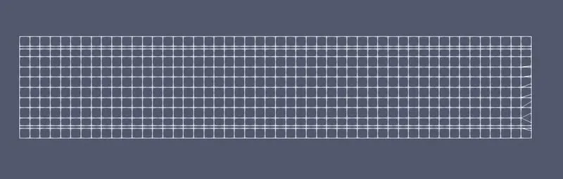
Mesh:
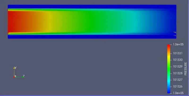
Pressure contour:
The link for pressure contour: https://youtu.be/xPvsJzcKk8E.
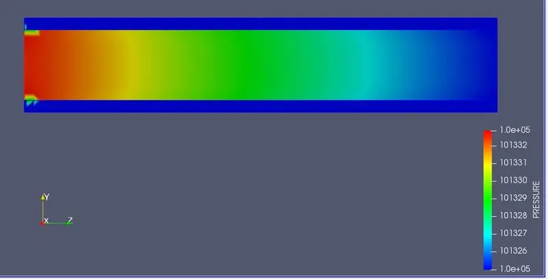
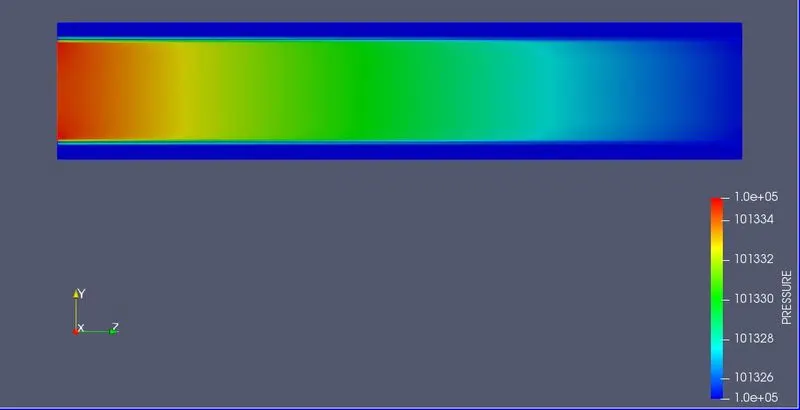
At time 0, a zero normal pressure gradient is set the inlet and 101325 Pa at the outlet. With the passage of time, we note the below profile. The inlet is at relatively high pressure when compared to the outlet. From the above plot it is noted that inlet which is an area of high pressure, corresponds to an area of low velocity, and outlet, which is an area of low pressure, corresponds to a high velocity.
Velocity contour:
The link for velocity contour: https://youtu.be/WAvGEimF9ZM
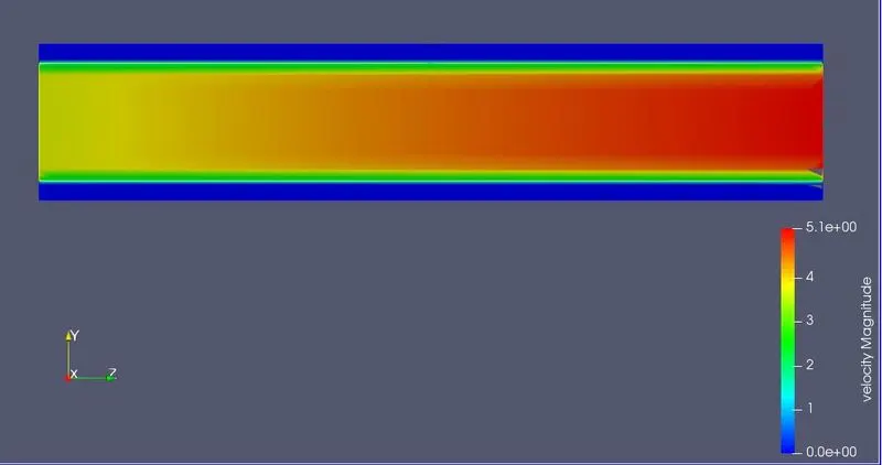
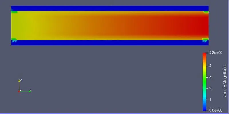
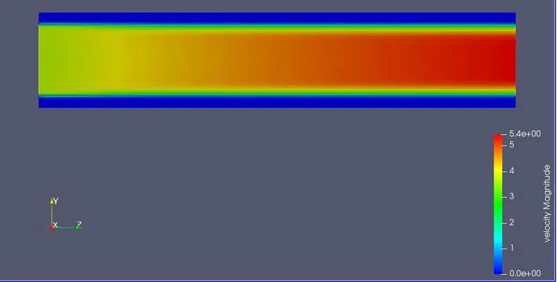
From the below plot, the development of the velocity profile is observed. At t=0, the velocity at the inlet is 3.661 m/s and the outlet is Om/s. Due to the pressure difference between the inlet and outlet, the flow gradually develops over time.
Temperature contour:
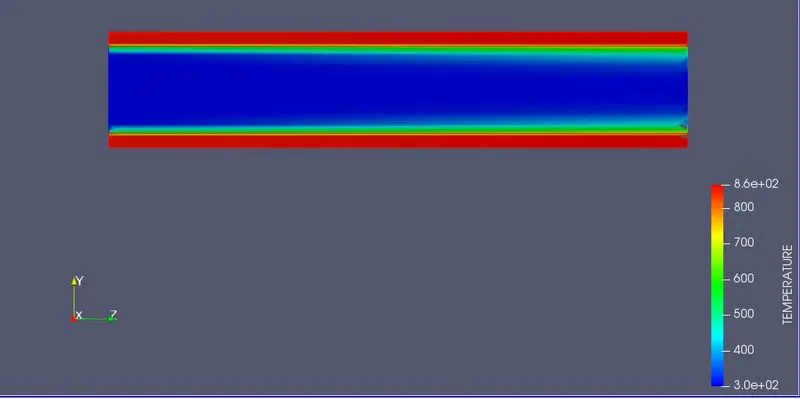
The link for temperature contour: https://youtu.be/yAl9q-xp5yg
Y-plus:
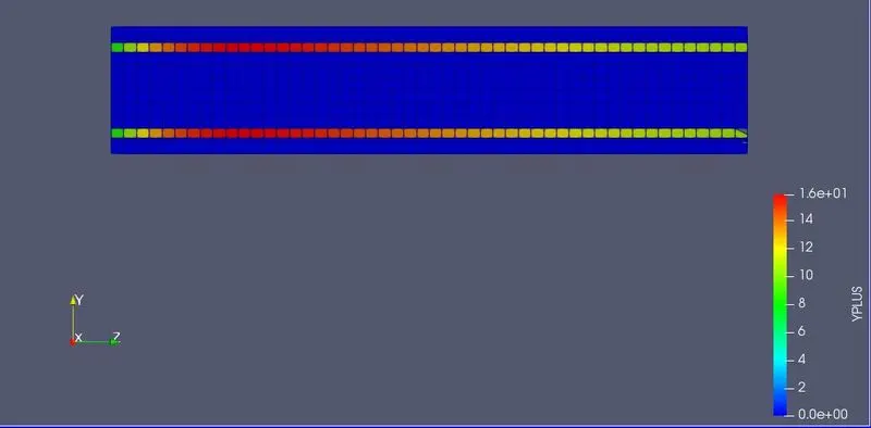
For the 2 refined grids of size 0.003m and 0.002m, a similar trend was observed as per the base mesh. They are commonly summarized at the end.
Case-2 (Base grid- 0.003 with super cycling 0.05):
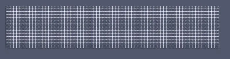
Mesh:
Pressure contour:
The link for pressure contour: https://youtu.be/nNR1kiGc62g
Velocity contour:
The link for velocity contour: https://youtu.be/A6pjuCGgK-M
Temperature contour:
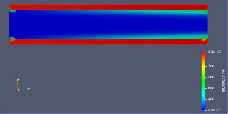
The link for temperature contour: https://youtu.be/ICZkgY554BA
Y-plus:
Case-3 (Base grid- 0.002 with super cycling 0.05):
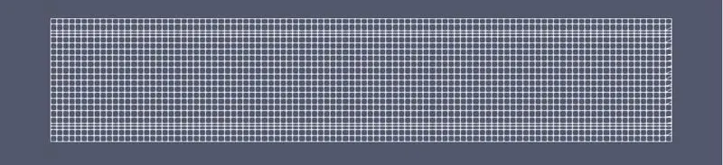
Mesh:
Pressure contour:
The link for pressure contour: https://youtu.be/4h6kJp-C774
Velocity contour:
The link for velocity contour: https://youtu.be/-Oe4iM6vIgc
Temperature contour:
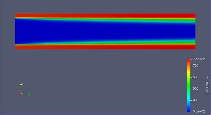
The link for temperature contour: https://youtu.be/IVADHh6J65c
Y-plus:
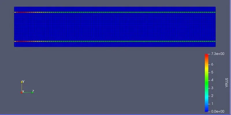
Comparison between different Meshes:
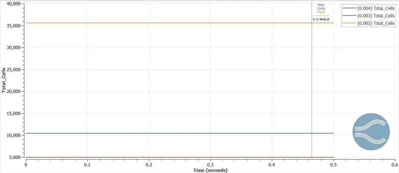
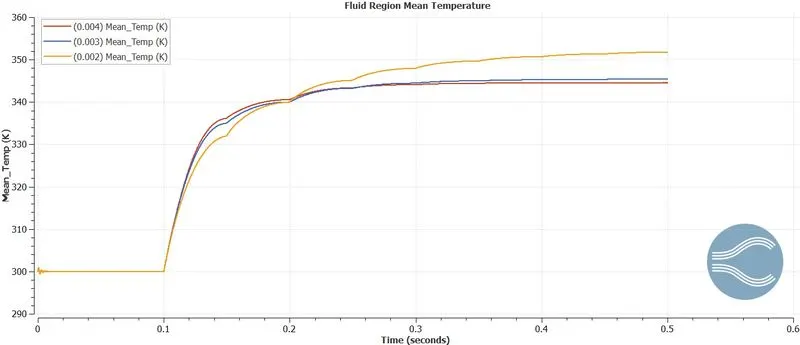
With the refinement of the grid it is seen that gradients in temperature, pressure are observed more clearly. However, there is a significant increase in computational time with refined mesh taking more time to arrive to a converged solution.
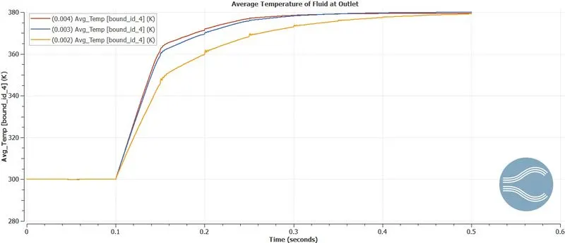
Outlet temperature converging to a particular value:
From the plot below we can see that the outlet temperature converges to the value of about 380 K.
Cell count and ranks:
Comparing the Fluid region mean temperature for different grid sizes:
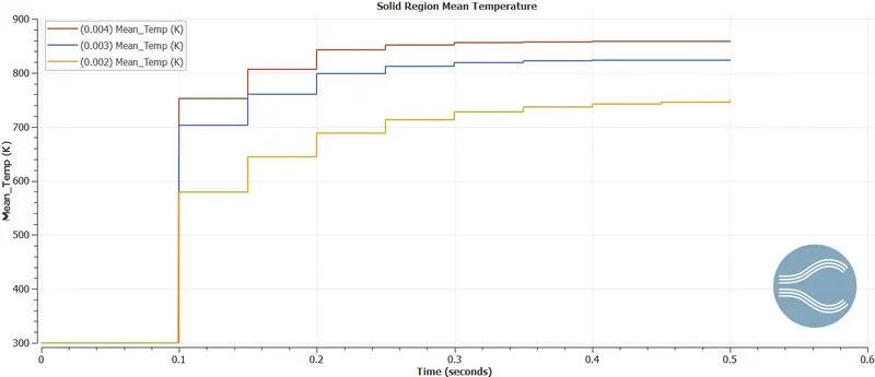
Comparing the Solid region mean temperature for different grid sizes:
Effect of super cycling:
Observations and Inferences:
The above shows how the simulation proceeds when the super-cycling time-length for each cycle stage is varied. As the time length is reduced, the solution converges at faster rates and reaches a steady value soon. The mean temperature converges very faster when the interval is 0.01s. As the time interval is increased the time taken to reach the steady-state increases. But in all the cases, the same final value is reached.
The time taken for the simulation for the various values of super cycling time interval are as follows:
1. For the 0.03s super cycling time interval the total simulation is 502.335761 seconds.
2. For the 0.02s super cycling time interval the total simulation is 471.834408 seconds.
3. For the 0.01s super cycling time interval the total simulation is 436.135848 seconds.