Week 1: Channel flow simulation using CONVERGE CFD
Channel Flow Simulation in Converge CFD:
Objective:
1. Creation of channel model in Converge CFD software.
2. Setup the case with appropriate material properties, boundary conditions, and different base grid sizes.
3. Run the simulation using the CYGWIN terminal. Plot mass flow rate, average velocity, and pressure plots using Converge software line plotting. Obtain velocity and pressure contours using ParaView software.
4. Interpret the results for different base grid sizes and follow it with a discussion.
Examples of channel flow are: pipe flow, closed rectangular channel flow, flow through an air duct, etc.
I.
Dimensions and Geometry:
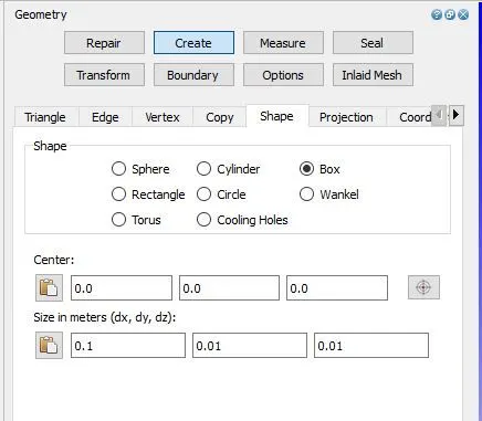
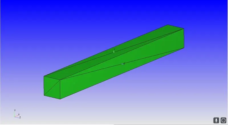
‘Geometry’ > ‘create’ > ‘shape’ > ‘box’ > and enter the values for center and dimensions and click ‘create’. The dimensions for the present geometry are shown in the figure along with the geometry.
Boundary Conditions:
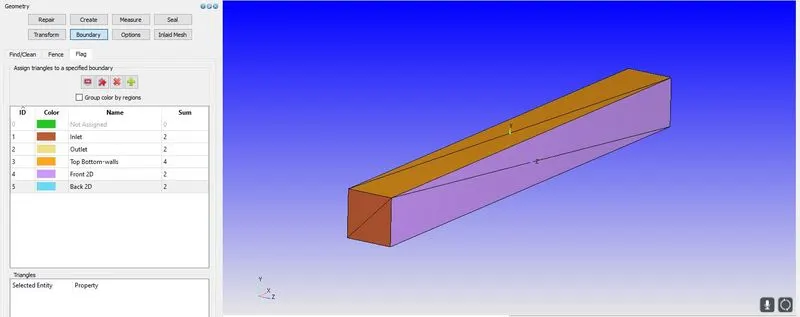
‘Boundary’ > click ‘+’ and select the required number of boundaries. Five boundaries are given for the geometry namely ‘Inlet’, ‘Outlet’, ‘Top Bottom-walls’, ‘Front 2D’, and ‘Back 2D’. Each of these assigned to the geometry as shown in the figure.
Orientation of normals:
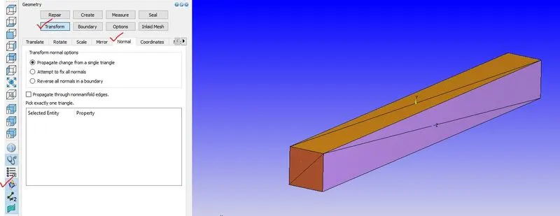
Here, initially, the normals are pointed outwards. In the channel flow case, fluid will pass inside the geometry and normals should be pointed towards the flow of fluid. Here normals are pointed outwards.
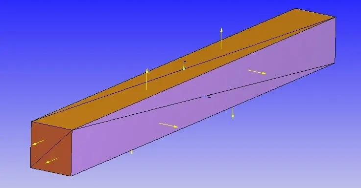
Click on ‘Transform’ > ‘Normal’ > ‘propagate change from a single triangle’, then select any triangle on the geometry and click ‘apply’.
Run Diagnosis:
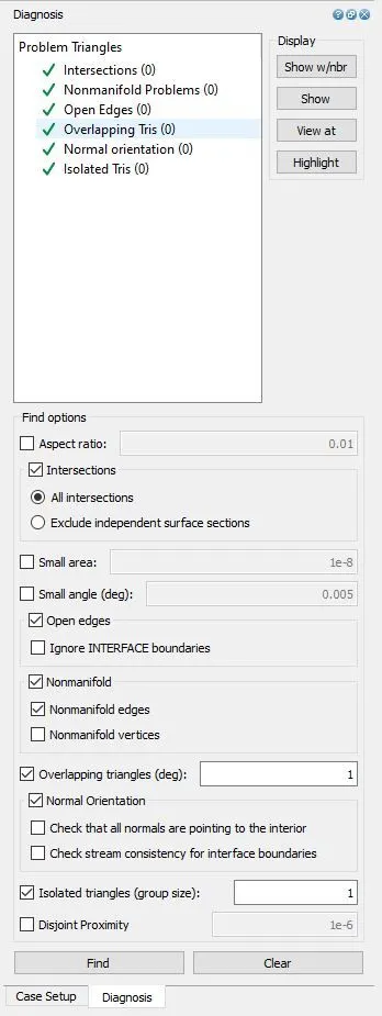
To check whether any problems exit during the above process of creating geometry, providing boundaries and normals, we run a diagnosis. The figure shows the diagnosis result and there are no errors present.
II.
1. Begin Case setup:
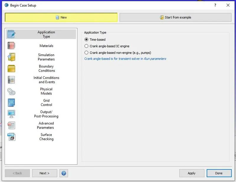
Application type: Time-based.
2. Materials:
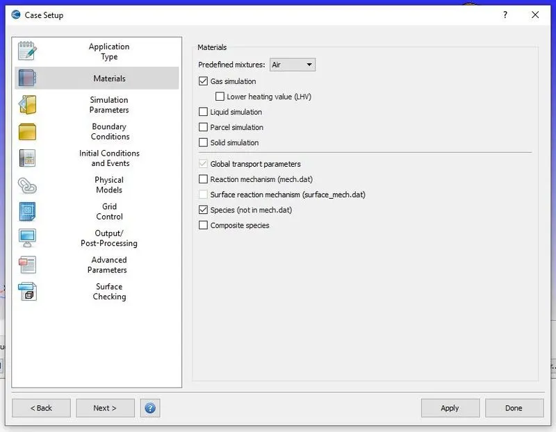
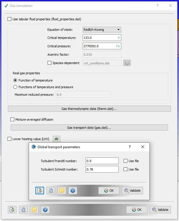
2.1: Gas simulation and 2.2: Global transport properties.
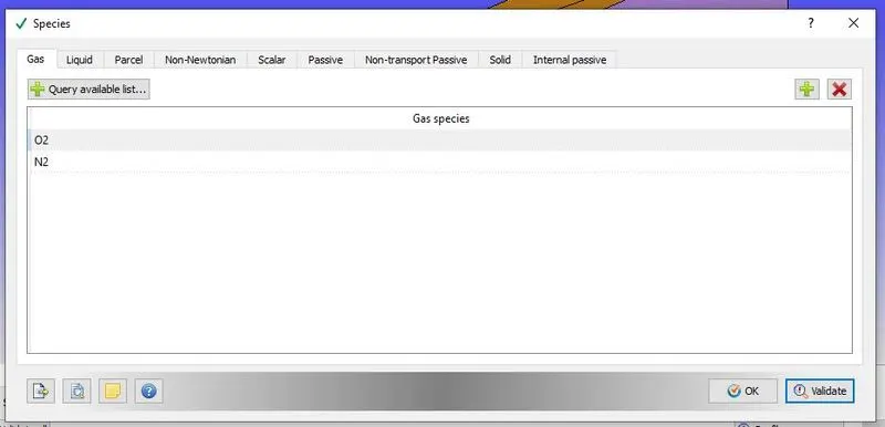
2.3: Species:
‘Gas’ > click ‘+’ > add oxygen and nitrogen.
3. Simulation parameter:
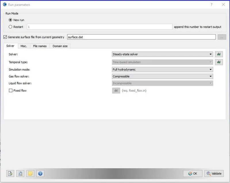
3.1: Run Parameters
Solver: Steady-state solver.
Simulation mode: Full Hydrodynamic (For simple geometry without complex and moving parts. Generation of mesh and solving of hydrodynamic equations are done).
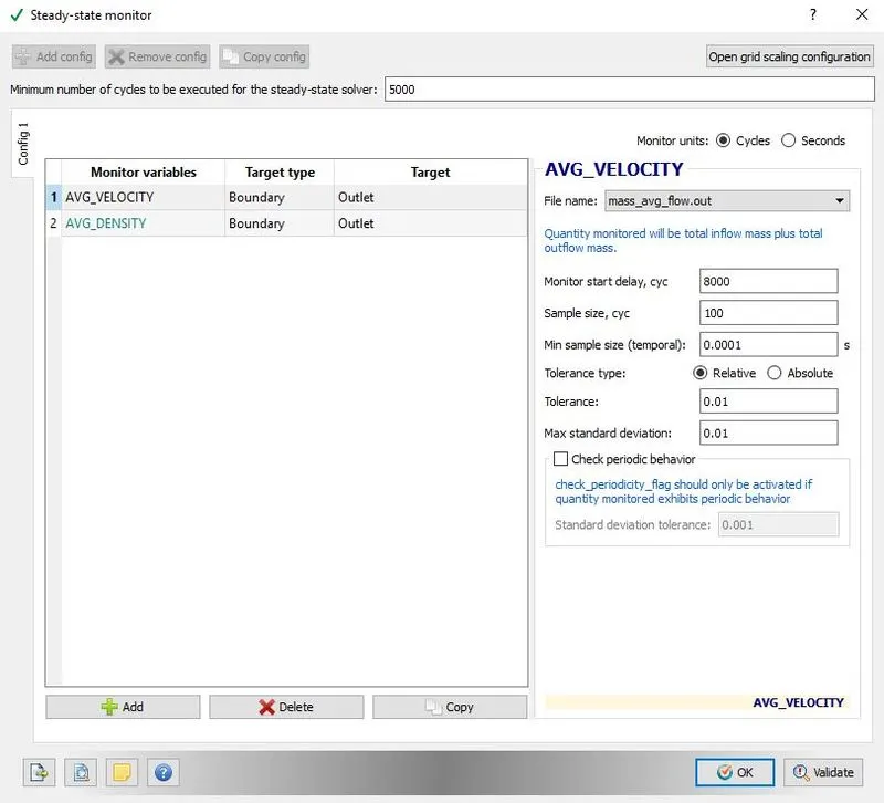
Misc: Tick: Steady-state monitor.
It will solve for a minimum number of 5000 cycles and check for convergence for every 100 cycles. Monitors variables should be given for checking. This helps us in reducing the time taken to run the simulation.
3.2: Simulation time parameters:
The number of cycles: 15000.
Note: Maximum convection CFL limit: 1.
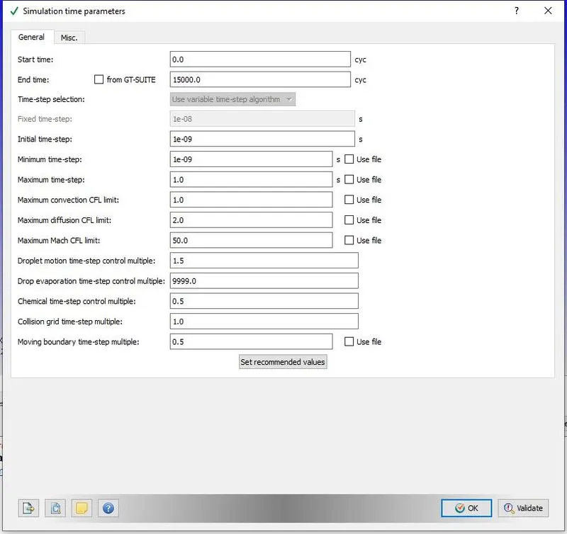
3.3: Solver parameters:
Navier-Stokes solver type: Density-based
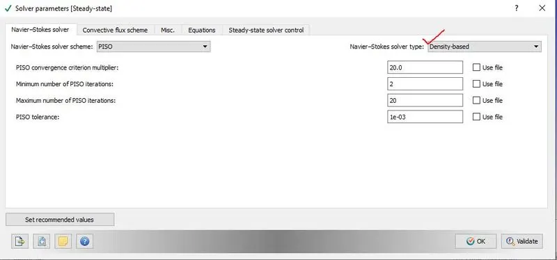
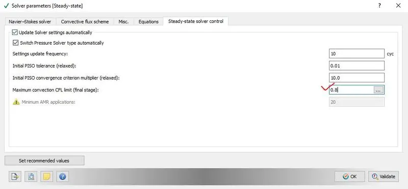
Maximum convection CFL limit should be set < 1. Here it is 0.8
4. Boundary Conditions:
‘Inlet’ > ‘Boundary Type: INFLOW’.
Pressure Boundary Condition: 100001 Pa. Add species in the ‘Species Boundary Condition’.
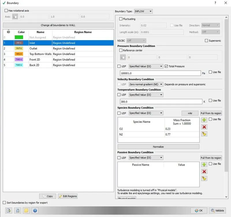
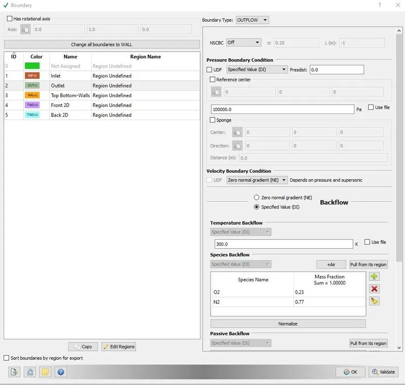
‘Outlet’ > ‘Boundary Type: OUTFLOW’.
Pressure Boundary Condition: 100000 Pa.
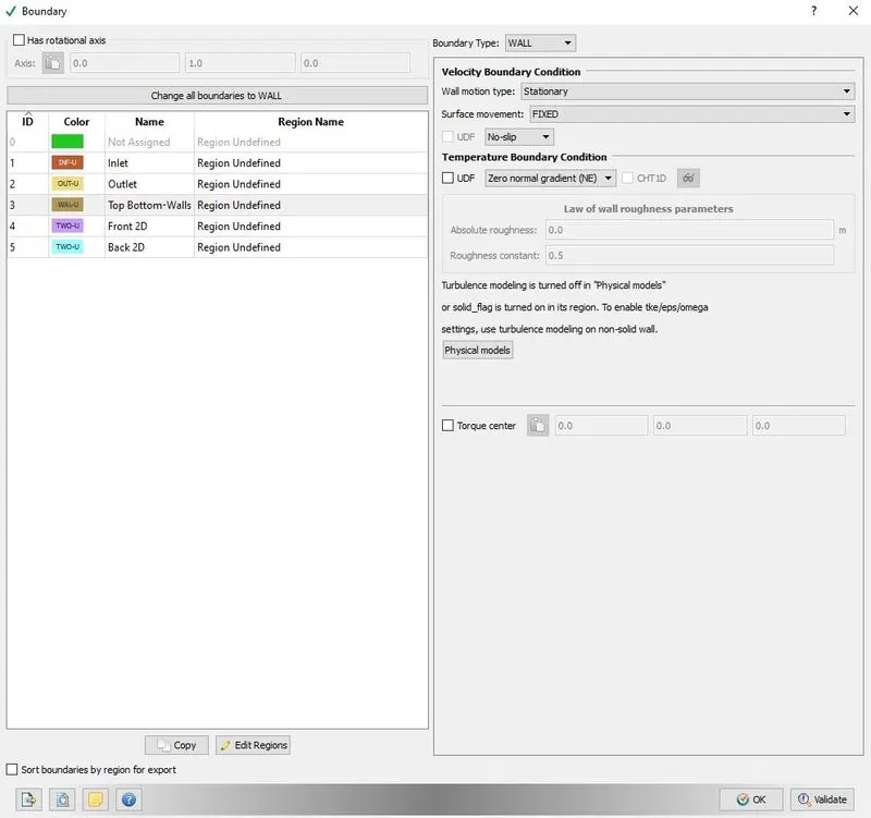
‘Top Bottom-walls’ > ‘Boundary Type: WALL’.
Select 'No-slip'.
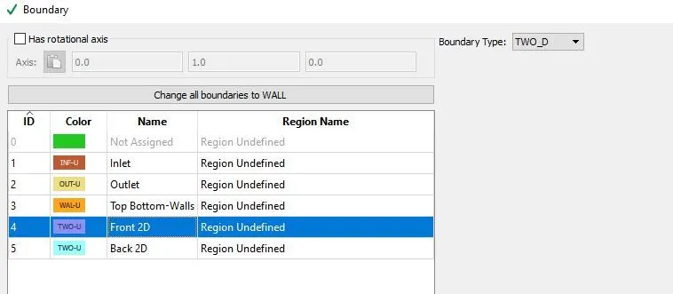
‘Front 2D and Back 2D’ > ‘Boundary Type: TWO_D’.
5. Initial Conditions and Events:
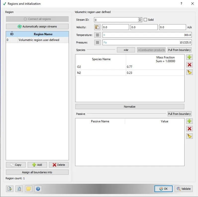
After this, go to ‘Boundary Conditions’ > ‘Region Name’ > ‘Volumetric region user defined’
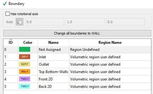
Then go to ‘Steady-state monitor’ > ‘Target’ > ‘Outlet’.
6. Physical Models:
Disable the turbulence modeling and click apply.
7. Grid Control:
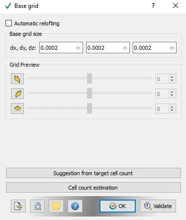
Case-1: dx: 2e-4, dy: 2e-4, dz: 2e-4.
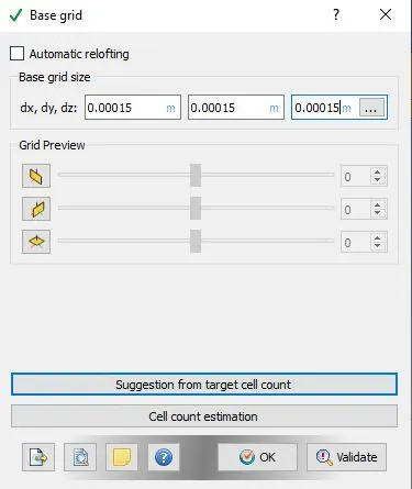
Case-2: dx: 1.5e-4, dy: 1.5e-4, dz: 1.5e-4.
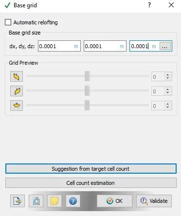
Case-3: dx: 1e-4, dy: 1e-4, dz: 1e-4.
8. Output/Post-Processing:
8.1: Post variable selection: Shown in the figure. Untick all related to combustion/turbulence.
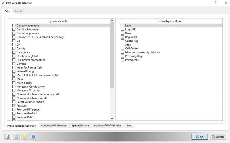
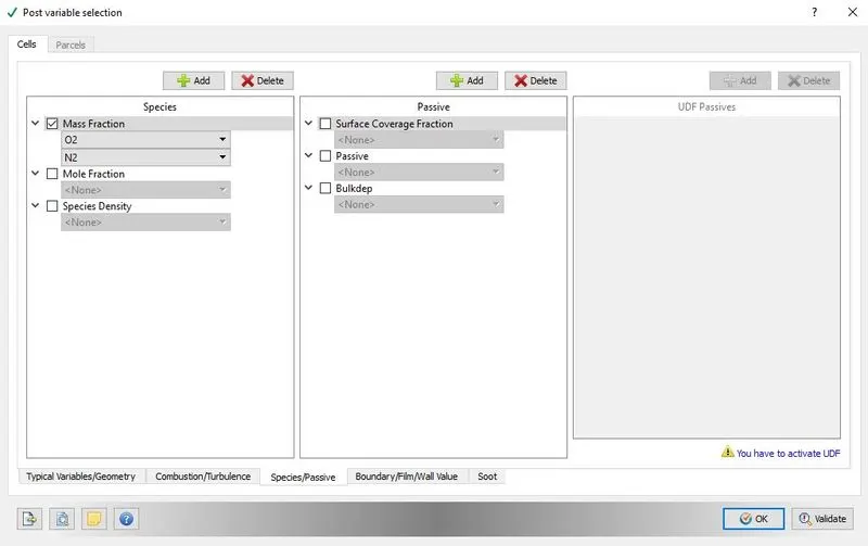
In ‘Parcels’ add O2 and N2 in ‘Mass Fraction’.
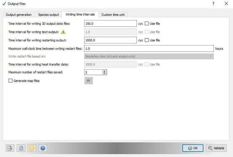
8.2: Output files:
End of Case Setup:
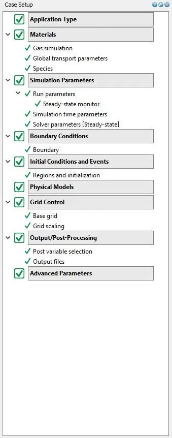
After this, we need to export the data. To do that, 'File' > 'Export' > 'Export input files'.
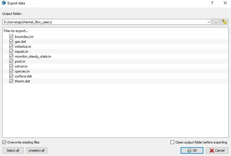
Case setup is completed.
III.
Running the simulation:
Open Cygwin and navigate to the folder in which the input files are exported and run the command as 'mpiexec.exe -n 4 converge.exe restricted' and then press enter. The simulation will run and in the end, if it shows 'normal termination', the simulation has ended successfully.
Post converting the output files:
We can do this in two ways. One way is to open CYGWIN and post-process. Another way is to do it directly in CONVERGE_Studio_v3.0. Here it is done in CONVERGE_Studio_v3.0.
On the bottom left side, click on post-convert. Give case name, in file type select: 'Paraview VTL in-line binary format'.
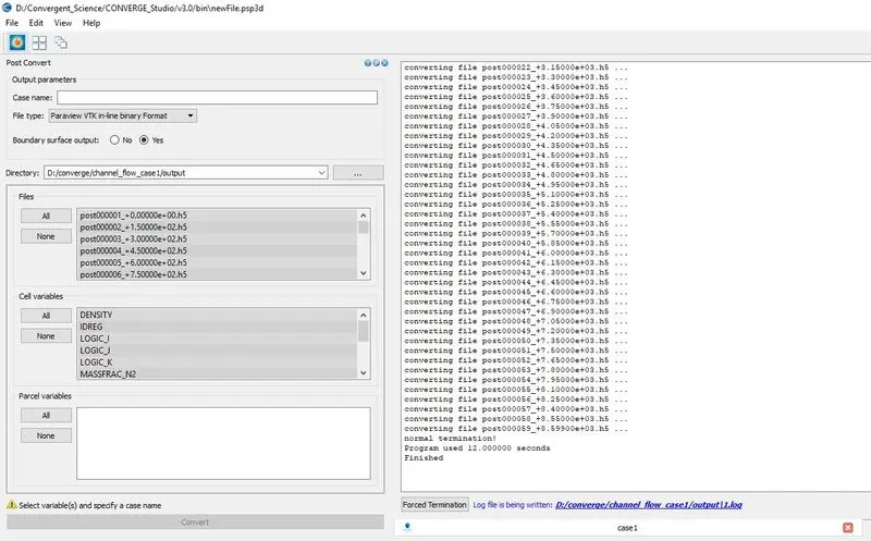
Results and Discussion:
Load up .vtm (set of files) files in ParaView software. Create a slice along the z-axis.
Case-1: Base grid size: dx=dy=dz=2e-4:
Mesh:
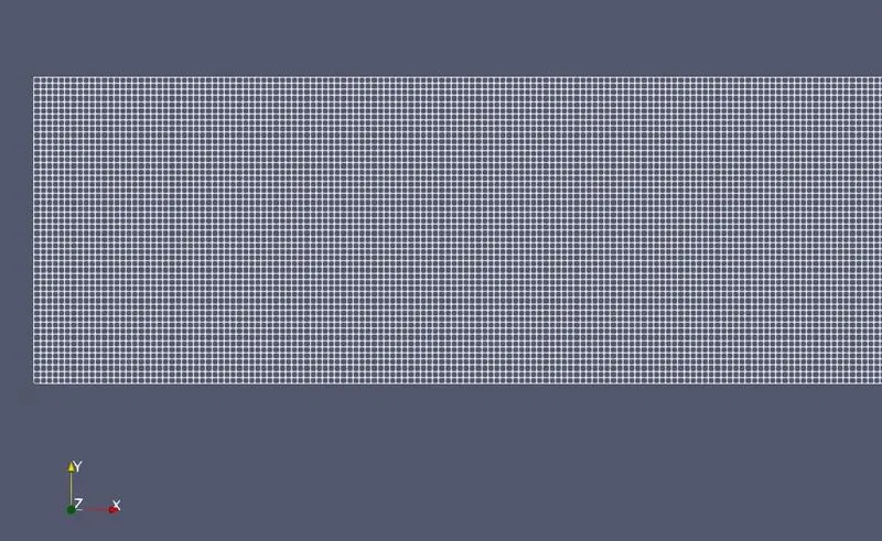
Velocity contour:
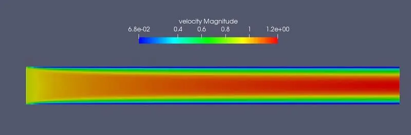
Link: https://youtu.be/RVrjdmjcMbk
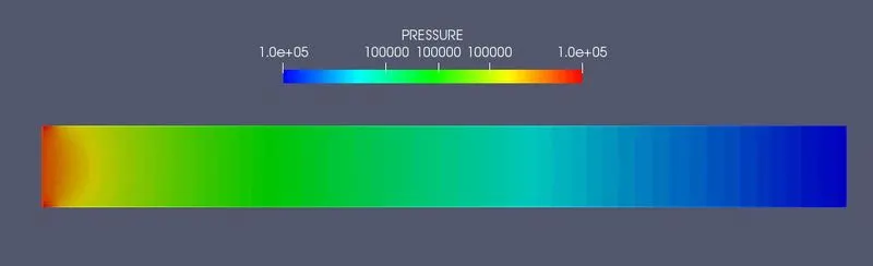
Pressure contour:
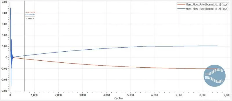
Mass flow rate plot:
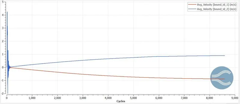
Average velocity plot:
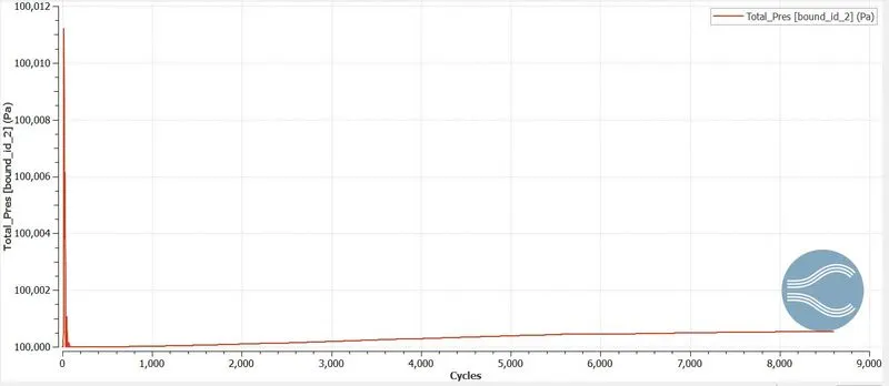
Pressure plot:
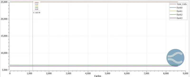
Total cell count:
Case-2: Base grid size: dx=dy=dz=1.5e-4:
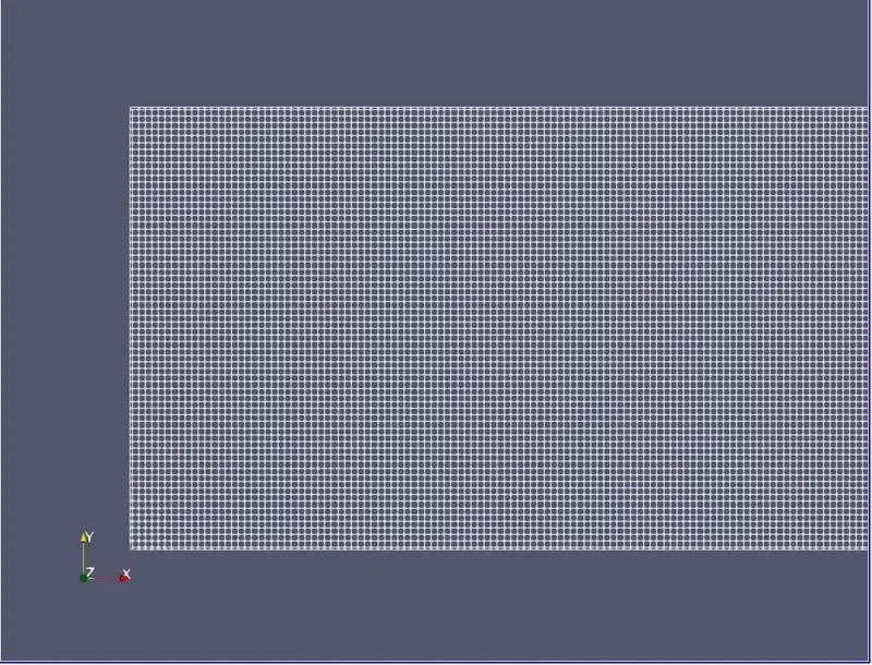
Mesh:
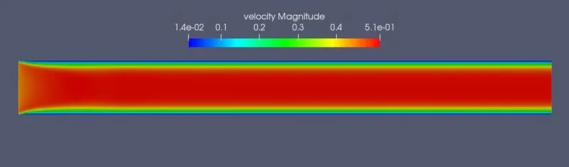
Velocity contour:
Link: https://youtu.be/9b-MrQcj9lg
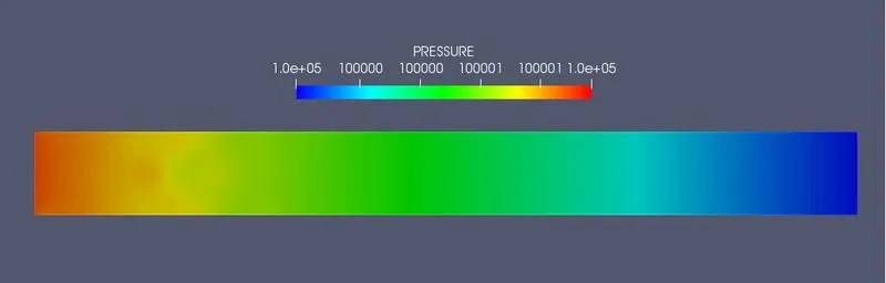
Pressure contour:
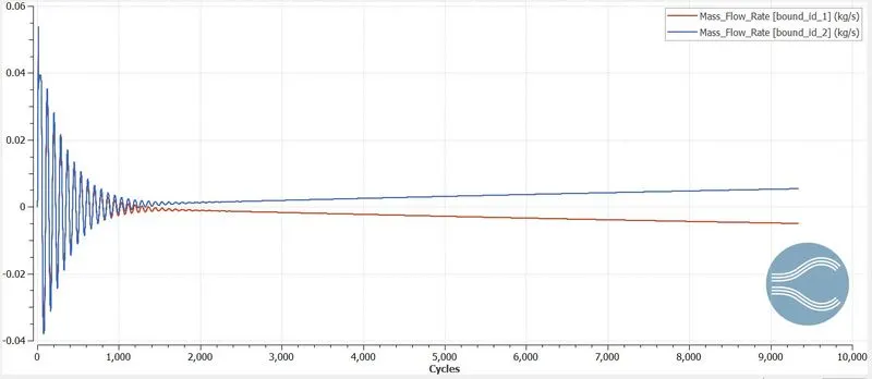
Mass flow rate plot:
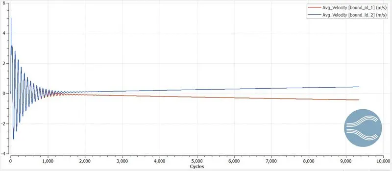
Average velocity plot:
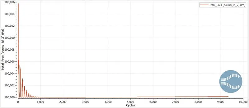
Pressure plot:
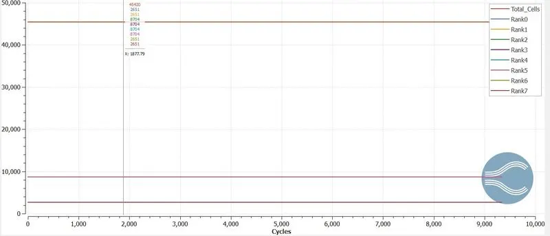
Total cell count:
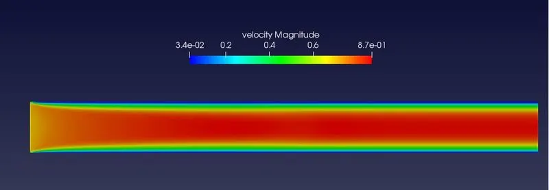
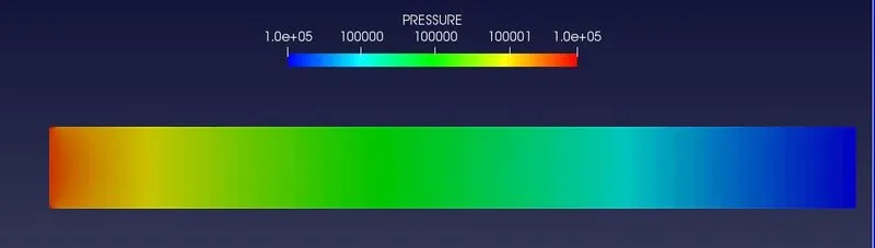
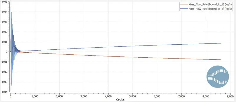
Case-3: Base grid size: dx=dy=dz=1e-4:
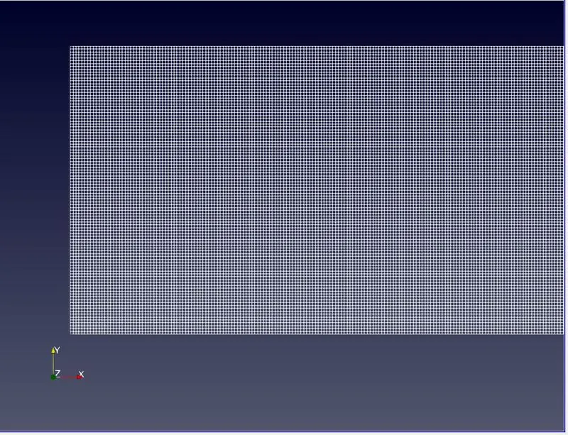
Mesh:
Velocity contour:
Link: https://youtu.be/-eI-tjNvOZs
Pressure contour:
Mass flow rate plot:
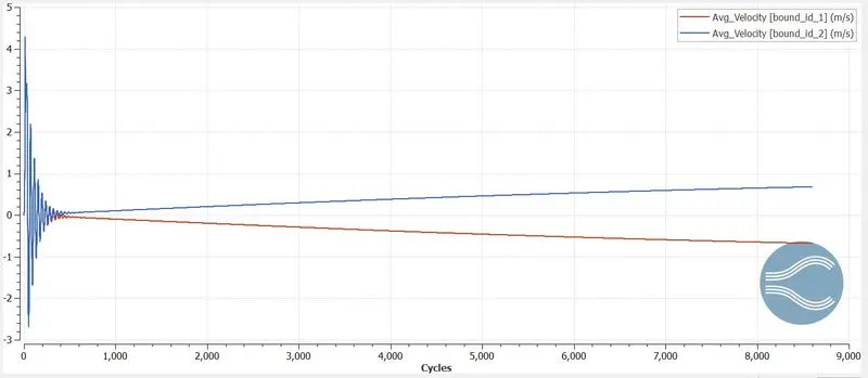
Average velocity plot:
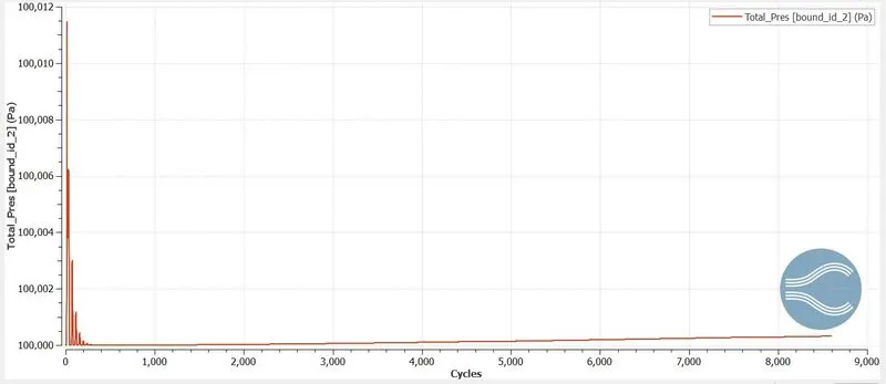
Pressure plot:
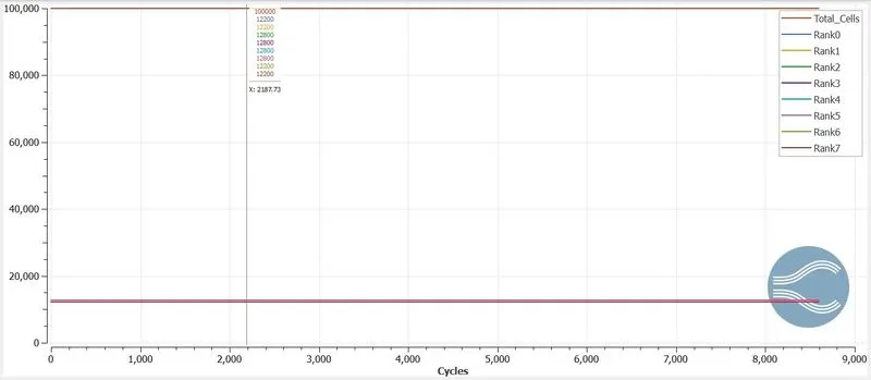
Total cell count:
Discussion:
In case-1 with dx=dy=dz=2e-4 base grid size, the total cell count is 25,000. For case-2 with dx=dy=dz=1.5e-4 base grid size, the total cell count is 45,420. For case-3 with dx=dy=dz=1e-4 base grid size, the total cell count is 100,000 . The velocity and pressure contours can be seen in the above figures for the respective cases. From the plots of mass flow rate, average velocity, and pressure, we can observe that as mesh becomes finer, the visibility of plots is getting better and smoother. Also with more cell count, the simulation time is getting longer but is giving more accurate results. One has to choose the correct base grid size required for their problem to save time and other resources while running simulation. There is a difference in velocity and pressure values in the contours for each grid size and this is to be noted.
The Pressure difference is the cause of fluid flow and can be seen in the above contours.
Also, the boundary layer phenomenon can be observed here. As the fluid enters the channel, there is the formation of a boundary layer and at the boundary wall, the fluid comes to a complete stop and assumes zero velocity relative to the surface wall due to no-slip condition. This is represented as the blue region in the velocity contours. The fluid layers, adjacent to the fluid layer sticking to the surface wall, also slow down and are seen as the green region in the velocity contours. As the flow continues in the channel, it reaches its maximum velocity (away from the surface wall) and is shown as the red region in the velocity contours.
Thank You.