Week 10: Project 1 - FULL HYDRO case set up (PFI)
Port Fuel Engine (PFI) FULL HYDRO Case Setup:
Objective (continuation from the previous project: https://skill-lync.com/student-projects/week-9-project-1-surface-preparation-and-boundary-flagging-pfi-17)
To Calculate:
1. The compression ratio of this engine.
2. Calculate the combustion efficiency of this engine
3. Use the engine performance calculator to determine the power and torque for this engine
4. Requirement of a wall heat transfer model.
5. Find out why can't we predict the wall temperature from the CFD simulation, and the significance of CA10, CA50, and CA90.
Proceedings:
Using the boundary flagging and mesh motion obtained from the no-hydro case, this project involves spray and combustion modeling to perform a full hydrodynamic case of Port Fuel Injection system. The case is simulated using a supercomputer and the output files are post-processed for engine characteristics.
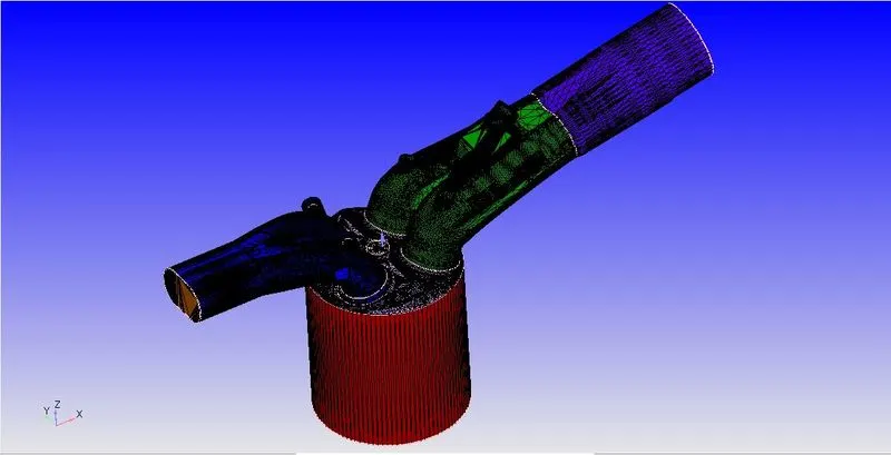
1. Engine Parameters:
Engine Geometric Parameters:
Bore=0.086 m
5troke = 0.09m
Etingrodlength = 0.18m
RPM = 3000
Run parameters:
Simulation mode: Full Hydro
Simulation time parameters: Start time: -520 deg, End time: 120 deg
2. Boundary Conditions (applied in converge):
Piston:
1. Boundary - WALL
2. Surface Movement - Moving
3. Temperature = 450K
4. Piston Motion - piston_profile.out
Inflow:
1. Boundary - INFLOW
2. Pressure 101325 bar
3. Temperature = 363K
4. Mixture - Air
Liner:
1. Boundary - Wall
2. Surface Movement - Fixed
3. Temperature = 450k
Cylinder Head:
1. Boundary - Wall
2. Surface Movement - fixed
3. Temperature 450 K
Exhaust Port:
1. Boundary - Wall
2. Surface Movement - Moving
3. Temperature = 450 K
Outflow:
1. Boundary-OUTFLOW
2. Pressure 101325 bar
3. Temperature = 800 K
4. Mixture - Air
5. CO2(mass fraction)- 0.192304
6. H2O(mass fraction) - 0.088559
7. N2(mass fraction) - 0.719137
Exhaust Valve Top:
1. Boundary - Wall
2. Surface Movement - Moving
3. Temperature = 525k
4. Profile - exhaust_lift.in
Exhaust Valve Angle:
1. Boundary - Wall
2. Surface Movement - Moving
3. Temperature = 525 K
4. Profile - exhaust_lift.in
Exhaust Valve Bottom:
1. Boundary - Wall
2. Surface Movement - Moving
3. Temperature = 525 K
4. Profile - exhaust_lift.in
Intake Port:
1. Boundary - Wall
2. Surface Movement - Moving
3. Temperature = 425 K
Profile - exhaust_lift.in
Intake Valve Bottom:
1. Boundary - Wall
2. Surface Movement - Moving
3. Temperature = 300 K
4. Profile - inlet_lift.in
Intake Valve Angle:
1. Boundary - Wall
2. Surface Movement - Moving
3. Temperature - 300 K
4. Profile - inlet_lift.in
Intake Valve Top:
1. Boundary - Wall
2. Surface Movement - Moving
3. Temperature = 300K
4. Profile - inlet_lift.in
Spark plug Terminal:
1. Boundary - Wall
2. Surface Movement - Fixed
3. Temperature = 600K
Spark Plug:
1. Boundary - Wall
2. Surface Movement - Fixed
3. Temperature = 600K
Intake Port
1. Boundary - Wall
2. Surface Movement - Fixed
3. Temperature = 425K
3. Initial conditions:
Intake port - 2 (closer to combustion chamber):
ic8h18 -0.025508
62 -0.20157
n2-0.77292
Temperature - 390k
pressure - 1 bar
Intake port - 1 (away from combustion chamber):
Air
Temperature - 370K
Pressure - 1 bar
Cylinder
Pressure - 1.85731 bar
Temperature - 1360K
Stoichiometric composition
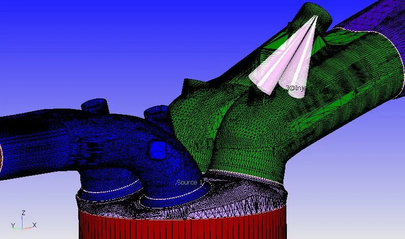
4. Spray Modeling:
CONVERGE includes state-of-the-art physical models for a wide variety of phenomena, including chemistry, turbulence, multiphase fluid flow, spray, and radiation, and it automatically couples these models so you don't have to. If you're looking for a shorter runtime, you can choose one of CONVERGE's simplified combustion models. If accuracy is paramount, CONVERGE's detailed chemical kinetics solver will help you obtain the results you need. For turbulence modeling, you can choose from a host of both RANS and LES models. For spray modeling, CONVERGE can capture physical processes from liquid injection and spray breakup to drop/wall interaction and evaporation. CONVERGE also includes several volumes of fluid modeling options to simulate multi-phase flows.
Select the spray modeling parameter in the physics models. In the spray modeling, we are using the O'Rourke model to initialize the spray of fuel. The species to be injected is selected as the fuel element IC8H18.
The following parameter values are introduced for the specifications of fuel injection.
Injection Parameters:
Fuel flowrate = 7.5e-4 Kg/second
Injection start time = -480.0
Injection duration = 191.2
Fuel temperature = 33OK
The Kelvin-Helmholtz (KH), Rayleigh-Taylor (RT) & Discharge coefficient models are being used for the injection. Here, we are using four nozzles for spraying the fuel into the cylinder with similar specifications as follows.
Nozzle positions:
Nozzle diameter = 250 mm
Circular injection radius = Nozzle radius
Spray cone angle = 10
Nozzle 0:
Center: 0.0823357 0.00100001 0.07019
Align Vector: -0.732501 0.210489 -0.647408
Nozzle 1:
Center: 0.0823357-0.00099999 0.07019
Align Vector: -0.732501-0.210489 -0.647408
Nozzle 2:
Center: 0.0823357-0.0004 0.07019
Align Vector: -0.5-0.2-0.647408
Nozzle 3:
Center: 0.0823357 0.0003 0.07019
Align Vector: -0.5 0.2-0.647408
5: Combustion Modeling:
CONVERGE'S SAGE detailed chemistry solver uses local conditions to calculate reaction rates based on the principles of chemical kinetics. This solver is fully coupled to the flow solver, but the chemistry and the flow solvers parallelize independently of one another, which speeds up the simulation. With the appropriate mechanism, the SAGE solver can predict a wide range of cases (e.g., a variety of fuels [premixed, non-premixed, partially premixed, multiple fuels], emissions modeling, and unique phenomena such as end-gas auto-ignition). With its accuracy and robustness, CONVERGE can perform predictive modeling instead of merely confirming experimental results.
The next step in the modeling is the combustion modeling parameter. The values for the combustion properties like start time, end time & species are to be specified as given in the image below.
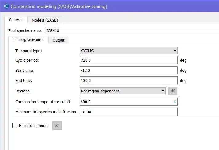
The combustion model here is taken as the SAGE model. The turbulence model is taken as the RNG K-Epsilon model.
6. Spark Ignition Parameters:
Start of spark = -15deg
Spark duration = 10deg
Spark location= -0.003 0 0.0091
Spark radius = 0.0005m
7. Grid:
The grid size is taken to be 0.004 m and fixed embeddings are done at critical points.
The valve angles are provided with a scaling of 3 as they are moving so close to the walls of the cylinder head. The mesh inside the cylinder is also refined to a scale of 2 as the combustion can be captured properly.
Fixed Embedding:
To refine that critical area, we can use Fixed Embedding around the Throttle Boundary. Fixed embedding is used to refine the grid at specific locations in the domain where a finer resolution is critical to the accuracy of the solution. Fixed embedding allows the rest of the grid to remain coarse to minimize simulation time.
Note that fixed embedding is given for: Intake Valve angles, Exhaust Valve angles, Big Cylinder embedding, Small cylinder embedding, Spark (Spherical embedding, Larger spherical embedding), and Injector embedding.
Adaptive Mesh Refinement:
Adaptive mesh refinement is done to capture the places at which the properties of the calculation are critical.
Note that the refinement is made to be adaptive for velocity and temperature. The parameters for both the properties are specified so that the mesh adapts the values from the specification to refine the places where the values tend to be within the specified parameter.
Post-processing results:
1. Max Pressure plot:
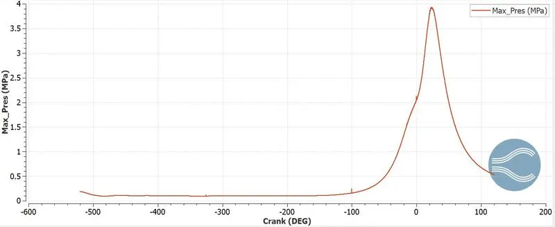
From the pressure plot, we can see that the pressure only varies a little until the ignition occurs. Once the ignition starts, the pressure inside the combustion chamber increases at a faster rate and reaches a maximum value when the chamber volume is minimum. Then after the power stroke, the piston moves apart increasing the volume which in turn decreases the pressure to the initial value.
2. Mean Temperature plot:
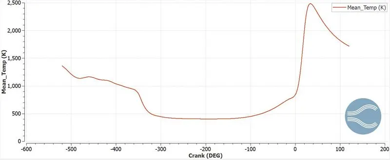
The temperature graph at the beginning has a low temperature which gets decreasing further as after an exhaust stroke the high-temperature emissions take place by decreasing the temperature inside the chamber. Once the chamber gets all the exhaust gas out, the temperature inside the chamber remains unchanged for a certain period of time until the ignition starts. Once the source of heat is released to the fuel particles from the spark plug, the temperature spreads to all the fuel particles thereby increasing the temperature inside the chamber.
3. Volume plot:
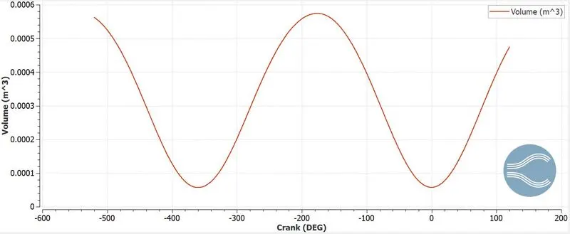
The volume of the combustion chamber follows a uniform waveform where the volume increases and decreases at the same rate. The piston follows a linear too & fro motion which controls the volume of the combustion chamber.
4. Heat Release Rate plot:
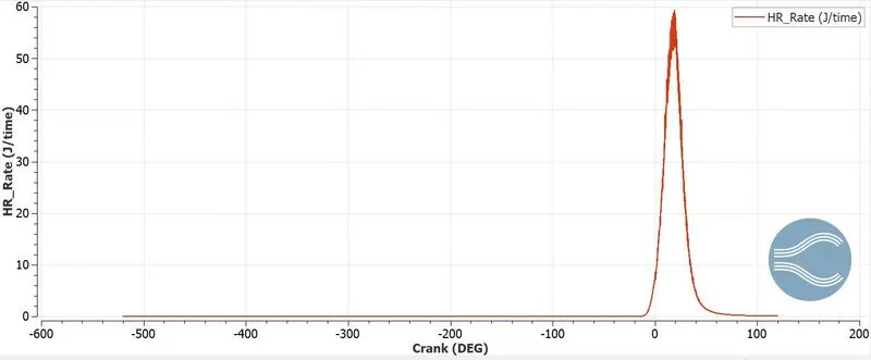
Heat Release Rate (HRR) is the rate at which fire releases energy - this is also known as power. HRR is measured in units of Watts (W). Depending on the size of the fire, HRR is also measured in Kilowatts (equal to 1,000 Watts) or Megawatts (equal 1,000,000 Watts).
5. Integrated Heat Release plot:
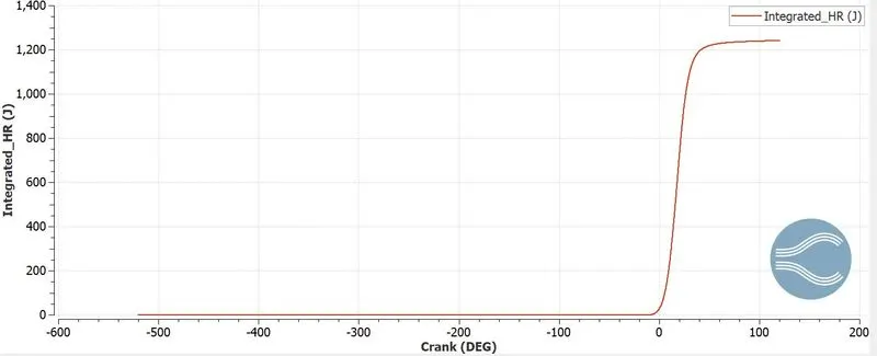
If we integrate the HRR plot we get this. Helps us calculate the amount of heat extracted inside the engine.
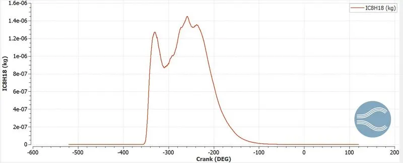
6. Fuel IC8H18 Spray plot:
7. Liquid Spray Drops plot:
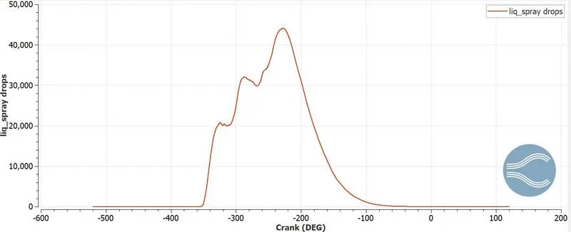
The maximum liquid droplets present in the cylinder is around 440000-450000. This decreases after some time due to evaporation and combustion. Eventually, this drops to a nearly zero value. From this, we infer that combustion is nearly complete in the cylinder.
8. Emissions plot:
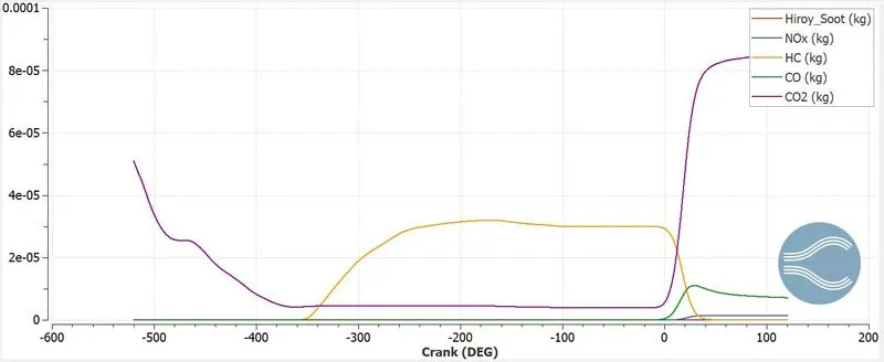
This plot shows us the amount of emission occurring in an IC Engine. We can see various materials of gas getting released at the exhaust port. The main gas particles are plotted in the graph above. We can see a high amount of CO2 emission at the end of the power stroke. The NOX emissions can also be read through this graph and proper actions can be taken if there are any emissions higher than the limited amount.
Calculations:
Compression Ratio of Engine:
In a combustion engine, the static compression ratio is calculated based on the relative volumes of the combustion chamber and the cylinder, that is, the ratio between the volume of the cylinder and combustion chamber when the piston is at the bottom of its stroke, and the volume of the combustion chamber when the piston is at the top of its stroke. The dynamic compression ratio is a more advanced calculation that also takes into account gasses entering and exiting the cylinder during the compression phase. The compression ratio is a fundamental specification for combustion engines. In a piston engine, the static compression ratio (CR) is the ratio between the volume of the cylinder and combustion chamber when the piston is at the bottom of its stroke, and the volume of the combustion chamber when the piston is at the top of its stroke.
From the 3. Volume plot:
Maximum volume = `5.74121xx10^-4` `m^3`
Minimum volume = `5.75786xx10^-5` `m^3`
`CR = (5.74121xx10^-4)/(5.75786xx10^-5)`
Compression Ratio: 9.971
Combustion Efficiency:
From the 5. Integrated Heat Release plot, the heat released is 1241.06 J.
Mass of fuel= `3xx10^-5`kg, calorific value= 43.4 MJ/kg.
`eta_(combustion)= 1241.06/(3xx10^-5xx43.4xx10^6)xx100`
`eta_(combustion)` = 95.21%.
Engine Power and Torque:
From Engine Performance Calculator,
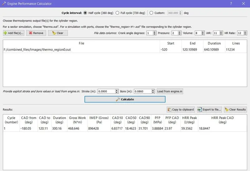
`W = 468.646`.
`N= 3000/60rps`. So `N = 50rps`.
Therefore the number of cycles completed in one second is 50. One degree of rotation completed = `1/(50xx360)`.
Time taken for 240.199 degrees is `1/[50xx360]xx240.199``
Power= `P = W/t (W)`= `frac[468.646xx50xx360][240.199]`.
Power= 35.119 KW.
To calculate torque, we make use of `P=(2pi NT)/60` where `T`= Torque.
So, `35.119=frac[2xxpixx3000xxT][60}`
`T=111.788`N-m.
Significance Of CA10. CASO & CA90:
However, to understand precisely the combustion status in different DFD modes, the parameters CA10 and CA50, and CA90 are specified here. The CA10 and CA50 are defined as the position of the crank angle (deg) at which the cumulative heat release reaches 10% and 50%, respectively. The physical significance of CA10 is that it is used to identify the start of ignition in a diesel engine, whereas the CA50 indicates the end of premixed combustion and the start of diffusion combustion of fuel used in the engine. The physical significance of CA10 is that it is used to identify the start of ignition in a diesel engine, whereas the CA50 indicates the end of premixed combustion and the start of diffusion combustion of fuel used in the engine. The higher the difference between CA10 and CASG (CA50-CA10), the higher will be the combustion duration and vice versa.
Requirement of a Heat Transfer Model:
In the CFD simulation of the PFI engine, the thermodynamic data of the species is provided as the input data which is used to predict the reaction rate of species in the domain and temperature change of species. But the thermodynamic data of the solid parts of the engine is not provided as input data for combustion simulation. Hence, the wall temperature of solid parts of the engine is not predicted in combustion simulation. Thus, a heat transfer model is required to predict the wall temperature of solid parts of the engine where thermodynamic properties of solid are provided as the input data. The conjugate heat transfer model predicts the temperature of the wall due to the interaction between the burnt species and solid parts of the engine.
Why can't we predict the wall temperature from the CFD simulation?
In IC engine analysis, the mass, momentum, and energy conservation equations in the regions are solved using the turbulence and combustion model. As we are more interested in the fluid region and not the solid region, we treat the walls as adiabatic. This helps in arriving at a convergent solution using less computational resources without affecting the combustion characteristics. It is to be noted that heat equations are found to converge much faster than that of the solids, and treating walls as adiabatic helps us save time. For studying the wall temperature, CHT analysis is performed by initializing the wall material with a suitable heat transfer coefficient. Using this, the heat loss from through the walls is determined and the combustion efficiency calculated again.
Mesh contour animation:
Temperature contour animation:
Pressure contour animation:
Piston and Parcel movement contour animation: