Week 5: Prandtl Meyer Shock problem
Aim and Objectives:
To simulate the Prandtl Meyer Shock flow in Converge CFD.
1. Simulate the supersonic and subsonic flow through a duct having a sharp corner.
2. Study the formation of shock waves in the duct.
3. Observe the effect of the SGS parameter on shock location and cell count.
Theory and Introduction:
What is a shock wave?
Shock is a type of propagating disturbance that moves faster than the speed of sound in that medium. It carries energy and can propagate through a medium similar to an ordinary wave. But in shock wave, there is an abrupt change in pressure, temperature, and density of the medium. It is a strong pressure wave in any medium air or water. It is created by supersonic aircraft, explosions, lightning, or other phenomena that create violent changes in pressure. Their speed increases as the amplitude is raised. The amplitude of a strong shock wave, as created in the air by an explosion, decreases almost as the inverse square of the distance until the wave has become so weak that it obeys the laws of acoustic waves.
Prandtl-Meyer expansion fan:
A Prandtl-Meyer expansion fan also known as a supersonic expansion fan which is a centered expansion process that occurs when a supersonic flow turns around a sharp corner or a convex corner. It consists of infinite Mach waves diverging from the sharp corner. Each wave turns the supersonic flow in small steps. A supersonic flow cannot turn through a single shock wave because that would violate the second law of thermodynamics.
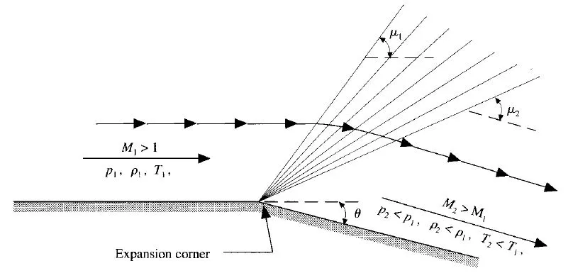 The above image shows the expansion fan (a set of diverging lines from the corner). As the flow passes through the expansion fan the velocity increases and thereby the Mach Number increases while the static pressure, temperature, and density decreases. This process is isentropic and that is why the stagnation properties (the total pressure and total temperature) remain constant across the fan.
Shock Flow Boundary Conditions:
• A boundary value problem is a differential equation together with a set of additional constraints called the boundary conditions.
• A solution to a boundary value problem is a solution to the differential equation which also satisfies the boundary conditions.
• A boundary value problem has conditions specified at the extremes of the independent variable in the equation.
Types of boundary conditions:
Dirichlet boundary condition:
In this type. When imposed on an ordinary or a partial differential equation, it specifies the values that a solution needs to take on
along the boundary of the domain.
Neumann boundary condition:
In this type, when imposed on an ordinary or partial differential equation, the condition specifies the values in which the derivative of a solution is applied within the boundary of the domain.
Robin boundary condition:
In this type, when imposed on an ordinary or a partial differential equation, it is a specification of a linear combination of the values of a function and the values of its derivatives on the boundary of the domain.
Mixed boundary condition:
In this type, a boundary value problem in which the solution of the given equation is required to satisfy different boundary conditions on disjoint parts of the boundary of the domain where the condition is stated.
Why Neumann boundary condition is used for a supersonic outlet?
Neumann b.c. is used because the values of all the variables like pressure, velocity, temperature, and Mach number are not available before solving the problem. So nothing is specified at a supersonic outlet and all variables are extrapolated from the domain interior. Only the normal derivative of variables is specified as zero gradient. If any pressure or velocity is specified at the outlet the solution will not converge and become unstable.
Geometry:
The deflection angle can be found out from the measure-angle option in converge geometry dock. The angle came out to be 5.64 degrees.
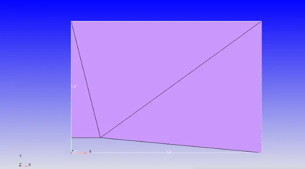
The boundary flagging is done like:
INLET, OUTLET, 2D-FRONT, 2D BACK, SLIP WALLS
The case set up:
Application type: Time based
On clicking apply, Converge studio by default loads values for the following groups Gas compressible steady flow.
1) Solver parameters
2) Steady-state monitor parameters
3) Simulation time parameters
• Materials:
The pre-defined mixture is selected as Air. The gas simulation box is checked. Species are turned on.
Under the Gas simulation tab, all the pre-loaded values are kept unaltered. Redlich-Kyong equation of state is used.
The turbulent Prandtl and turbulent Schmidt numbers are kept unchanged from the preloaded values.
In the species tab, under gas, The constituents of air, that is O2 and N2 are added.
Solver parameters:
A density-based solver is opted for. The Navier stokes Solver scheme is PISO. The maximum convection limit is set to 1.
• Boundary conditions:
1) INLET: Boundary type is inflow. The pressure boundary condition is specified value of 101000 Pa. Velocity Boundary conditions is Specified value(DI). The velocity in the x-direction is 680 m/s. The temperature boundary condition is also a Specified value(DI). The temperature at the inlet is 286 K. Species boundary condition is the specified value(DI). The species is air (O2,N2).
2. OUTLET: The boundary type is outflow. Supersonic condition prevails at the outlet. The pressure boundary conditions and the velocity boundary conditions at the outlet is Zero normal gradient (NE). The backflow temperature is also set to Zero normal gradient.
3.2D-FRONT: 2D boundary conditions
4. 2D-Back: 2D boundary conditions
5. Slip: Boundary is set to the wall type. Under the velocity boundary condition, the wall motion type is stationary and the surface movement is fixed. The temperature boundary condition is Zero normal gradient(NE).
• Region initialization:
A region is created with the name region0. Velocity in the x-direction is 680 m/s and the temperature is 286 K. the species is air. Every boundary is assigned to this region.
• Physical models:
Under the physical models, only turbulence modeling is required for this simulation. Turbulence modeling: Reynolds averaged Navier-Stokes (RANS) is selected.
• Grid control:
Under grid control, the base grid is auto-selected. In addition to that, adaptive mesh refinement is opted for. The base grid size is: dx = 0.8 m; dy=0.8 m;dz=0.8 m.
Adaptive mesh refinement:
In numerical analysis, adaptive mesh refinement (AMR) is a method of adapting the accuracy of a solution within certain sensitive or turbulent regions of simulation, dynamically and during the time the solution is being calculated.
In the adaptive mesh refinement, the maximum number of cells is limited to 200000. The region0 initialized, is transferred from available regions to active region. Temperature is checked.
Embed type= Sub-grid-scale (SGS) and the time control type is sequential. The maximum embedding level is 3.
The sub-grid criterion is changed in the subsequent simulations from 0.01 K to 0.05 K and 0.1 K.
Results:
Four cases were setup
Case 1: Velocity = 680 m/s (Supersonic flow) and SGS parameter = 0.01
Case 2: Velocity = 680 m/s (Supersonic flow) and SGS parameter = 0.1
Case 3: Velocity = 680 m/s (Supersonic flow) and SGS parameter = 0.05
Case 4: Velocity=100 m/s (Subsonic flow) and SGS parameter = 0.05
Case 1: Velocity = 680 m/s and SGS = 0.05:
Mesh:
Velocity:
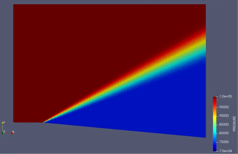
Pressure:
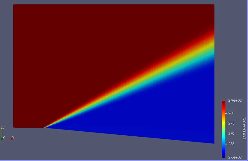
Temperature:
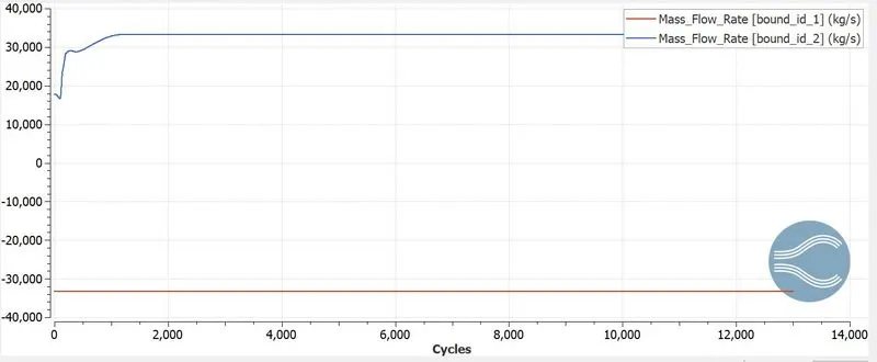
Mass Flow Rate:
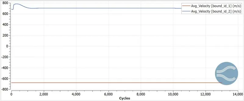
Average Velocity:
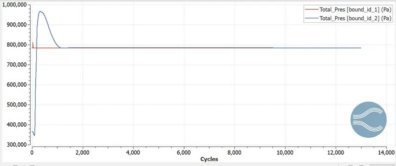
Total Pressure:
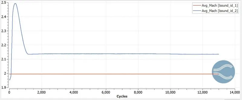
Average Mach:
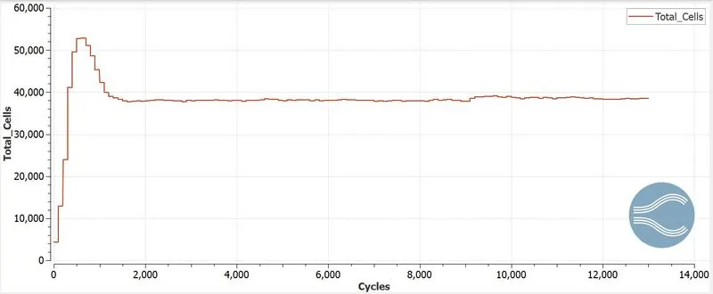
Total Cells:
Case 2: Velocity = 680 m/s and SGS parameter = 0.1
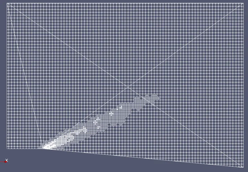
Mesh:
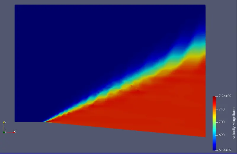
Velocity:
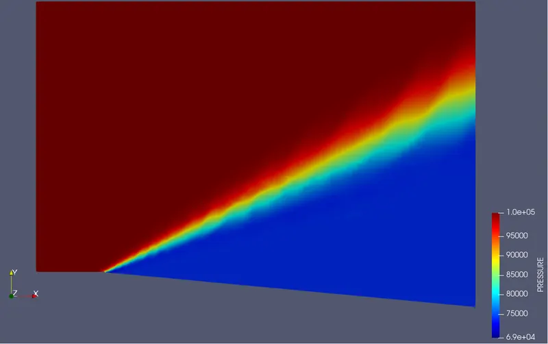
Pressure:
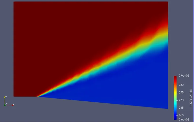
Temperature:
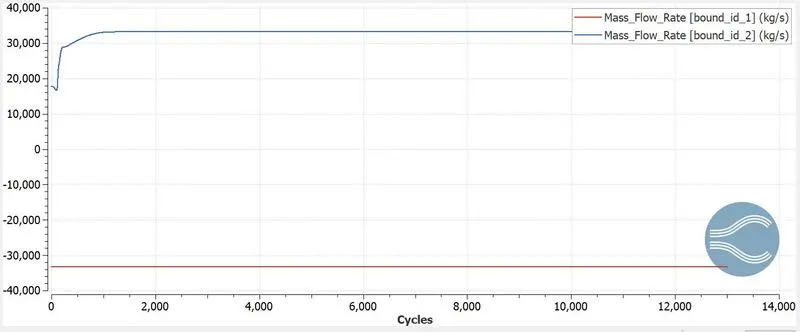
Mass Flow Rate:
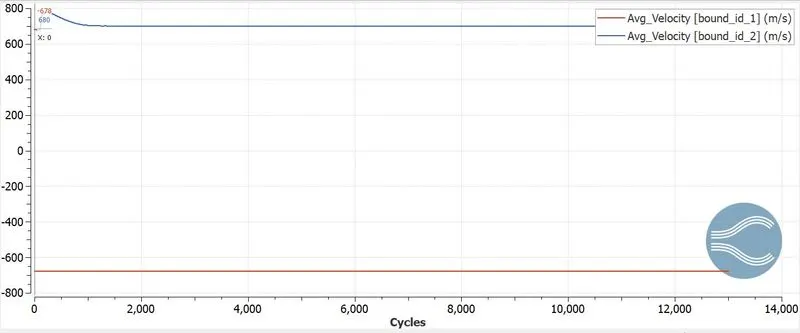
Average Velocity:
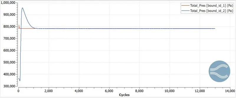
Total Pressure:
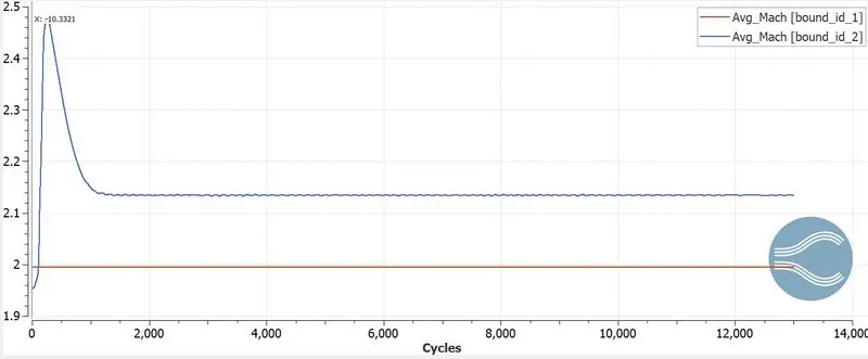
Average Mach:
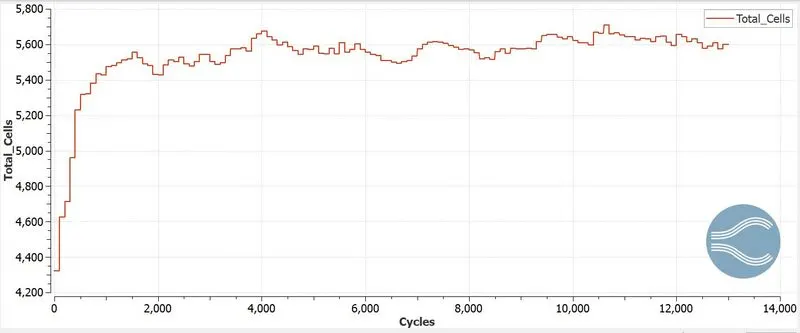
Total Cells:
Case 3: Velocity = 680 m/s and SGS parameter = 0.05
Velocity:
Pressure:
Mass Flow Rate:
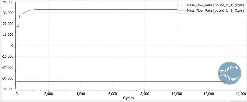
Average Velocity:
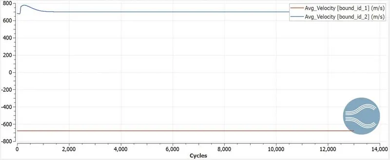
Total Pressure:
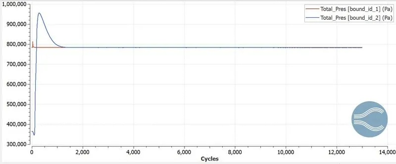
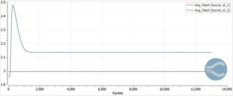
Average Mach:
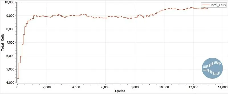
Cell Count:
Case 4: Velocity=100 m/s and SGS parameter = 0.05:
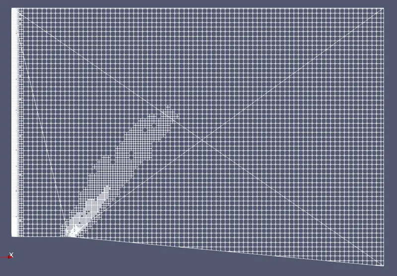
Mesh:
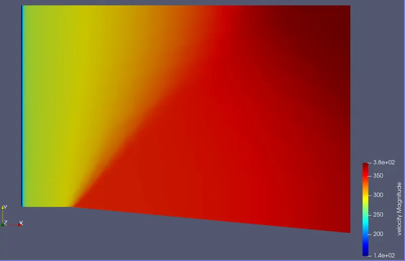
Velocity:
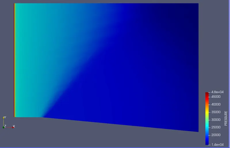
Pressure:
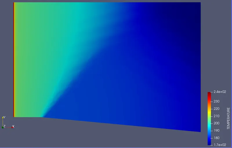
Temperature:
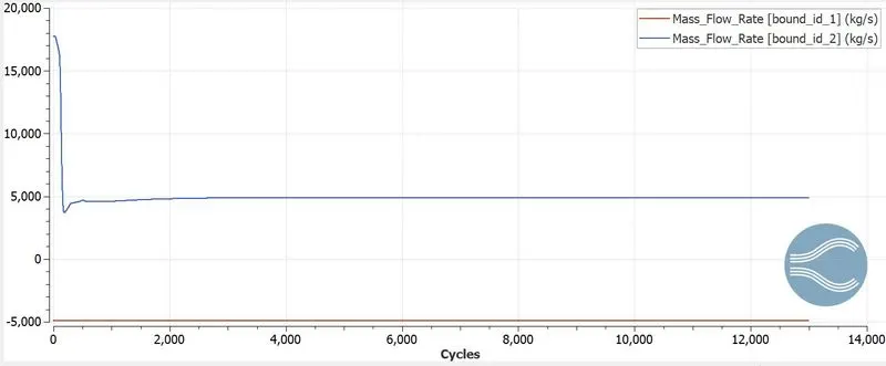
Mass Flow Rate:
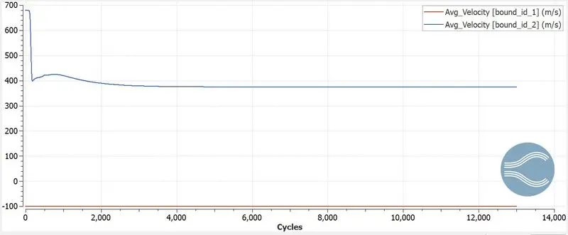
Average Velocity:
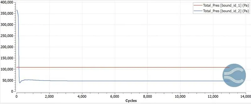
Total Pressure:
Average Mach:
Cell Count:
Observations and Conclusions:
Effect of SGS:
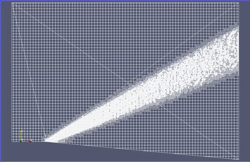
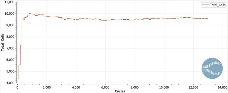
As SGS decreases, the total cell count increases. So that for small SGS parameter, AMR refines the mesh with more cells in and around the shock waves. For high SGS the mesh refinement area is very small whereas for small SGS the mesh refinement area is more. So for small SGS refinement spans from the sharp edge till the outlet boundary.
Subsonic vs Supersonic flow:
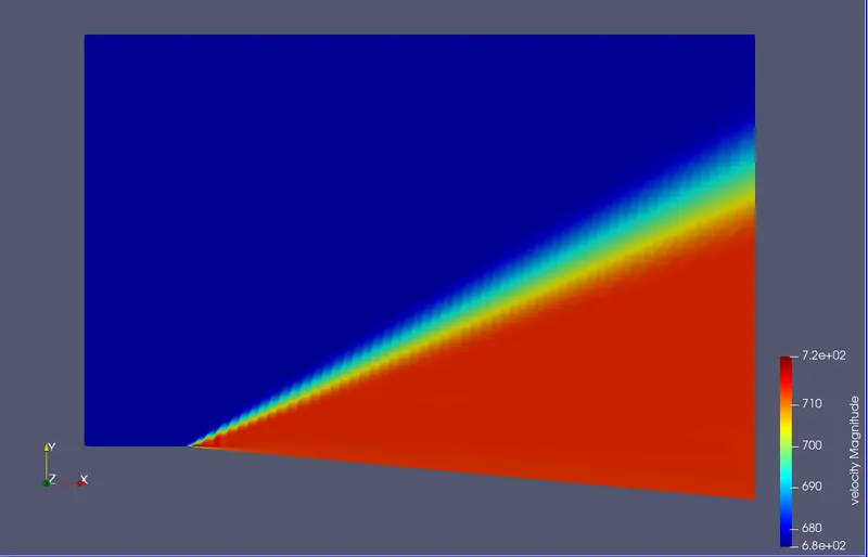
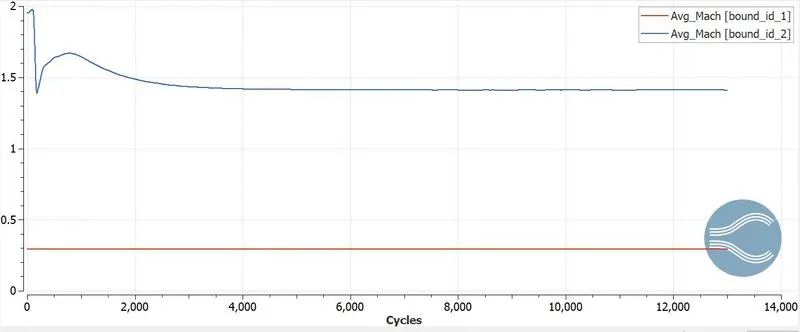
In supersonic flow, the Prandtl Mayer expansion fan is clearly visible and the mesh refinement is also visible in shock occurring regions. In subsonic flow. the Prandtl Mayer expansion fan is not visible and the mesh refinement is also not visible because there are no sudden fluctuations in parameters like pressure, temperature, velocity, and density. The average Mach number increases from inlet to outlet in the case of supersonic flow whereas in subsonic flow it decreases.
The simulation of supersonic and subsonic flow through a duct was set up and run in converge CFD. The various contour plots are studied for different cases. The formation of shock waves and the effect of SGS on the shock location was studied.