Week 1- Mixing Tee
Abstract:
Mixing Tee joints are widely used in the petrochemical, HVAC industry, etc. In this project two types of mixing tee joints are taken varying in length: short and long and simulated the flow of hot air and cold air through their inlets at different temperatures and different velocities according to the given momentum ratio. K-Epsilon and K-Omega models were used to simulate the airflow and were compared for a baseline simulation. Model producing the best results was used furtherly with a refined mesh. Surface reports for an area-weighted average of temperature and standard deviation of temperature are plotted at the outlet to obtain outlet temperature values and to understand the effectiveness of mixing respectively. Temperature and velocities contours were presented along with line plots and charts using post-processing. Finally, mesh independence test was carried out to determine the dependence of the results on the mesh density.
Objective:
Simulate hot and cold airflow in mixing tee of varying in length: short and long through their inlets at different velocities.
To test K-Epsilon and K-Omega models.
Velocity and temperature contour plots on the cut planes along and across the pipe and line plots along and across the length of the pipe.
Perform Mesh independent study for any one case.
Discuss the effect of length and momentum ratio on results.
Introduction:
In industrial process engineering, mixing is a unit operation that involves the manipulation of a heterogeneous physical system with the intent to make it more homogeneous. Mixing is performed to allow heat and/or mass transfer to occur between one or more streams, components, or phases. A mixing tee is a type of mixing mechanism. Mixing Tees utilizes a specifically engineered internal geometry to efficiently mix two fluid streams into one combined stream. Mixing tees are widely used in the petrochemical, HVAC industry, etc. in which two fluid streams with different physical and/or chemical properties mix together. Here in this case hot air flowing in the main pipe is mixed with cold air flowing through the tee. Selecting a suitable turbulence model between K-Epsilon and K-Omega is done. The velocity and temperature contours are presented. Residual plots and Line plots along and across the pipe were shown. Effect of length and momentum ratio were discussed. Finally, grid independence test is done.
Simulation Work:
1. Test K-Epsilon and K-Omega models:
Geometry:
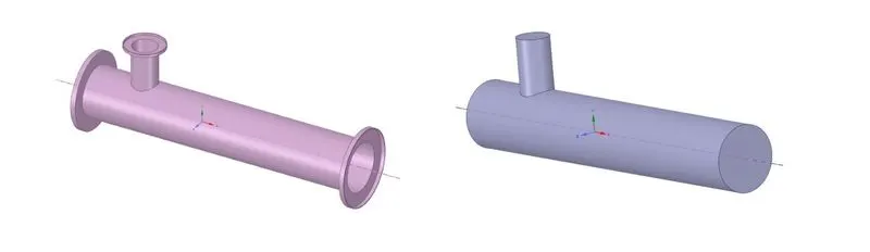
Loading up the geometry and volume extraction for the geometry is done using Ansys Spaceclaim in the Fluent module of the Ansys Workbench.
Short Mixing Tee geometry and volume extraction:
Meshing:
Meshing is done in Ansys workbench meshing in the fluent module. A baseline mesh of 1.0219e-002 m is used. Also named selections: Inlet-x, Inlet-y, Outlet, and Walls are given.
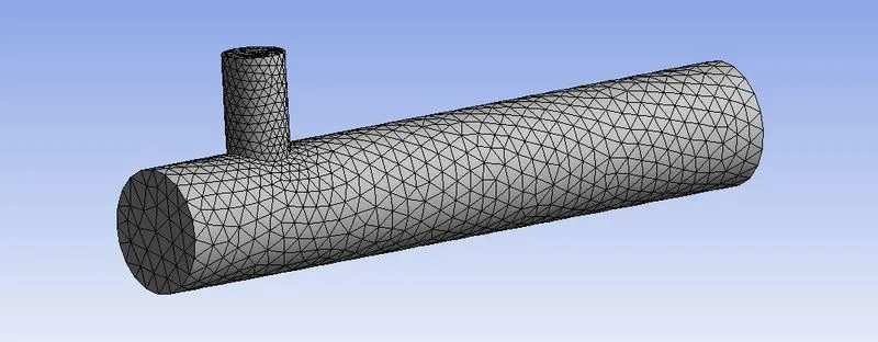
The number of elements: 13014.
Setup:
Checking of mesh is done. Steady-state, pressure-based, and absolute velocity formation solver is used. Energy is selected because measuring temperature is involved.
The models selected: K-epsilon realizable and K-omega SST.
Materials are selected. Cell zones and the same boundary conditions are given for both models.
Boundary conditions:
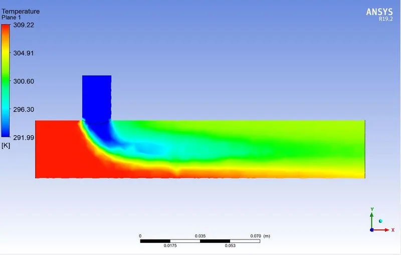
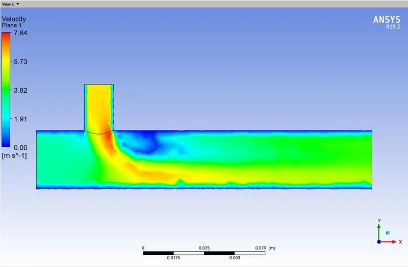
Inlet-x: Type-velocity inlet: Velocity of air= 3 m/s and Temperature of air= 309 K.
`Momentum ratio=(velocity of cold air)/(velocity of hot air)`
Taken momentum ratio =2. So the velocity of cold air is 6 m/s.
Inlet-y: Type-velocity inlet: Velocity of air= 6 m/s and Temperature of air= 292 K.
Outlet: Type-pressure outlet.
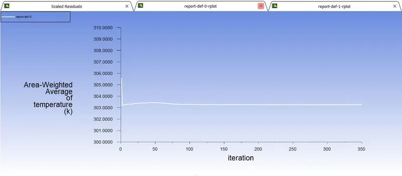
Definitions: Area weighted average and Standard deviation for temperature are plotted.
Initialization: Hybrid
The number of iterations: 350.
Results:
Temperature and velocity contours of K-epsilon model:
Temperature and velocity contours of K-omega model:
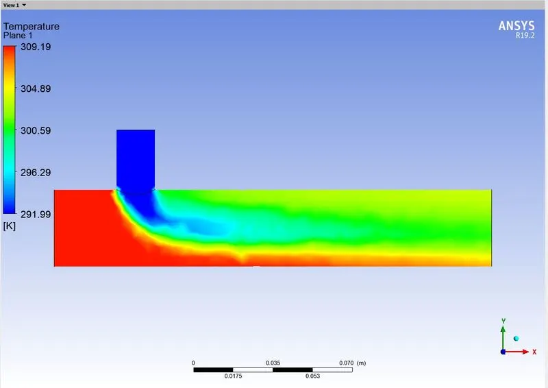
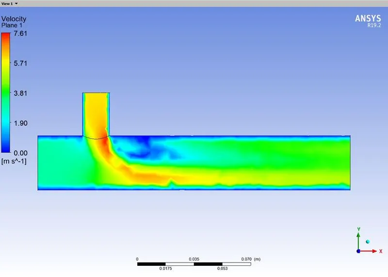
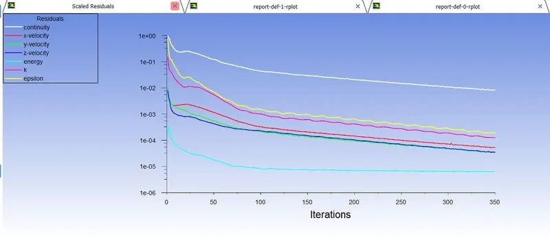
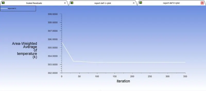
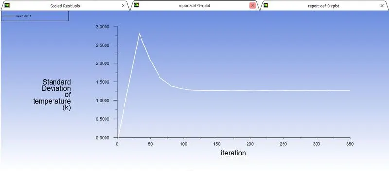
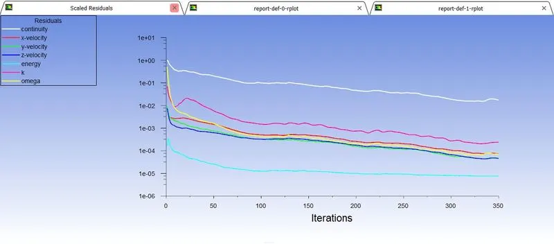
Residual plot, and Area-weighted average and standard deviation of temperature plots of K-epsilon model:
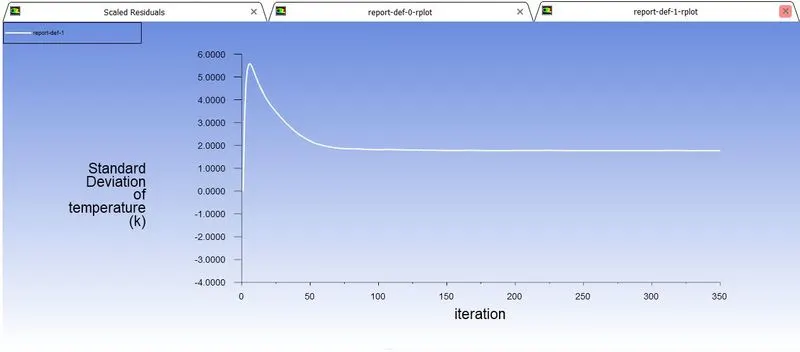
Residual plot, and Area-weighted average and standard deviation of temperature plots of K-omega model:
Observations:
The K-omega model is well suited for simulating flow in the viscous sub-layer. On the contrary, The K-epsilon model is ideal for predicting flow in the regions away from the wall.
In this particular case we are not dealing with walls, therefore, we are going to use the k-epsilon method for further simulations. Also For momentum ratio 2 the standard deviation of the K-epsilon model is lower than the K-omega model. Hence the K-epsilon model has a better mixing efficiency than the K-omega model.
We proceed with the K-epsilon model.
2. Case Setups:
2-a: Short mixing tee (momentum ratio: 2).
Geometry:
Loading up the geometry and volume extraction for the geometry is done using Ansys Spaceclaim in the Fluent module of the Ansys Workbench.
Meshing:
Meshing is done in Ansys workbench meshing in the fluent module. Element size of 0.002 m is used. Also named selections: Inlet-x, Inlet-y, Outlet, and Walls are given.
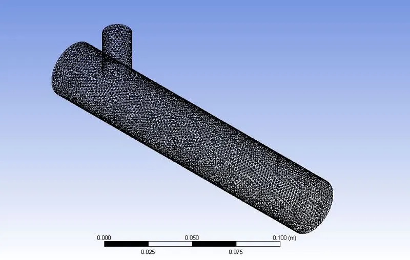
The number of elements: 106916.
Setup:
Checking of mesh is done. Steady-state, pressure-based, and absolute velocity formation solver is used. Energy is selected because measuring temperature is involved.
The models selected: K-epsilon realizable.
Materials are selected. Cell zones and the same boundary conditions are given for both models.
Boundary conditions:
Inlet-x: Type-velocity inlet: Velocity of air= 3 m/s and Temperature of air= 309 K.
`Momentum ratio=(velocity of cold air)/(velocity of hot air)`
Taken momentum ratio =2. So the velocity of cold air is 6 m/s.
Inlet-y: Type-velocity inlet: Velocity of air= 6 m/s and Temperature of air= 292 K.
Outlet: Type-pressure outlet.
Definitions: Area weighted average and Standard deviation for temperature are plotted.
Initialization: Hybrid
The number of iterations: 500.
Results:
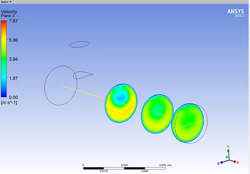
Temperature and velocity contours:
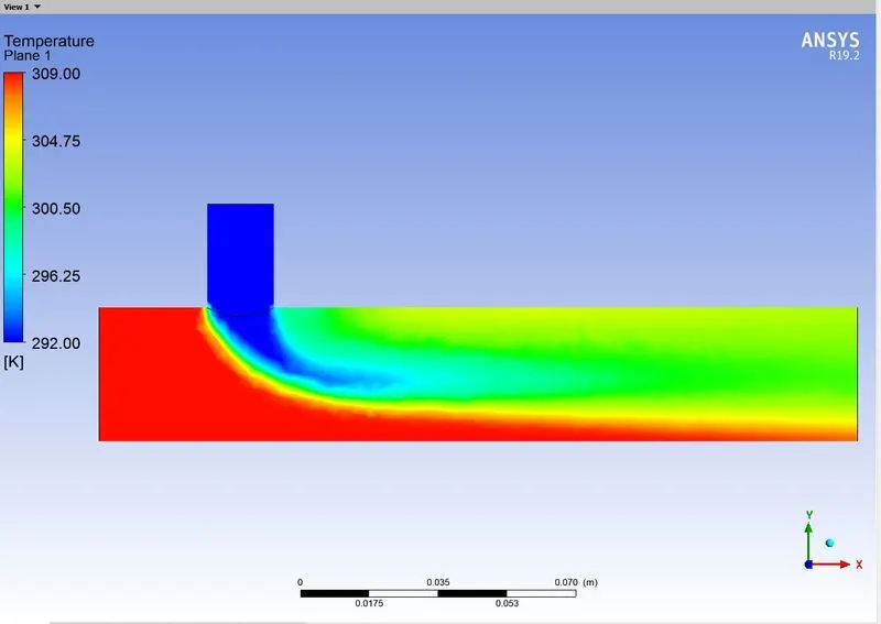
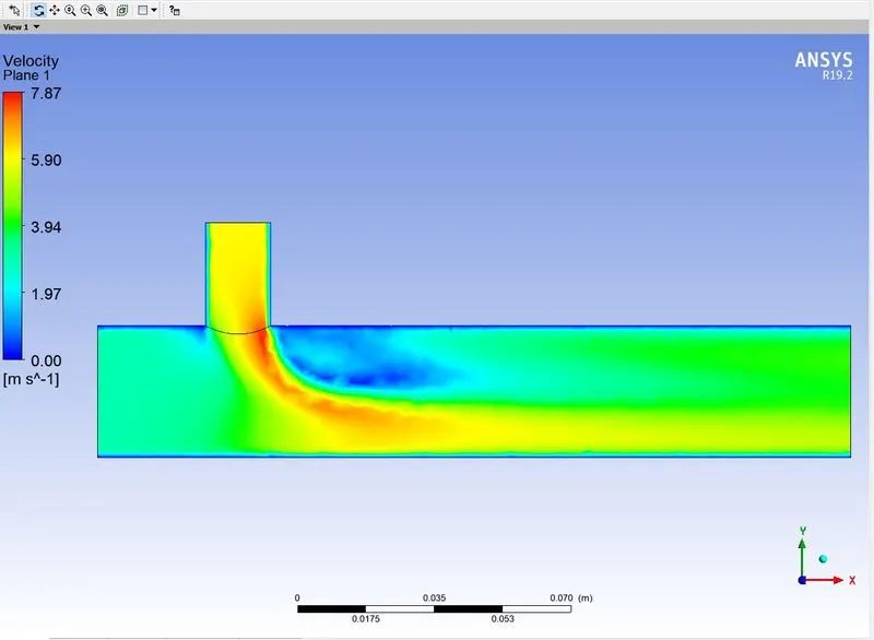
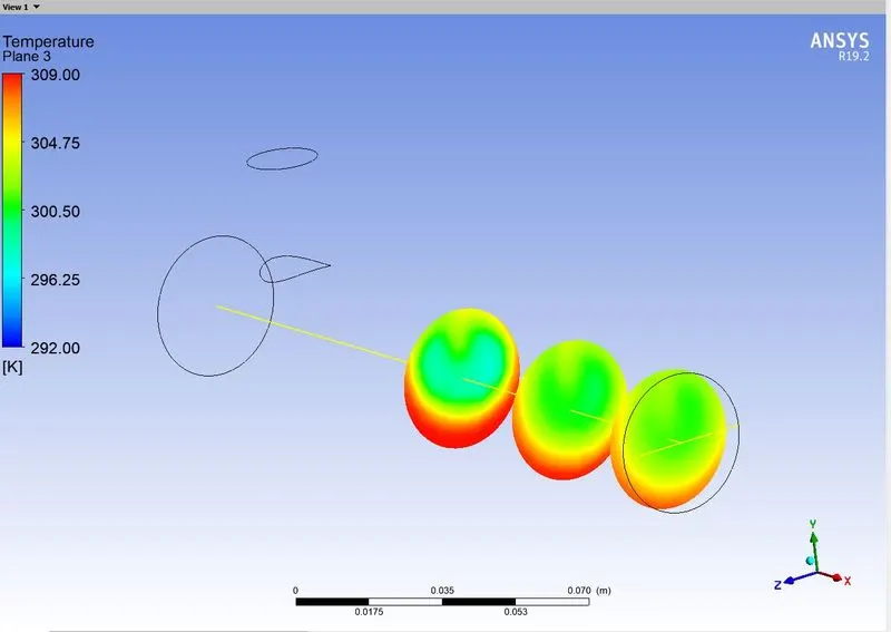
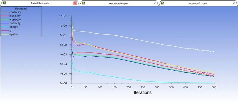
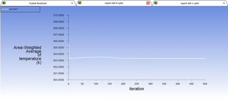
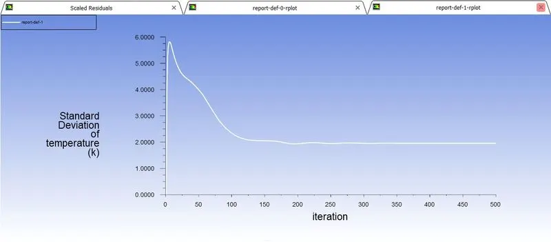
Residual plot, and Area-weighted average and standard deviation of temperature plots:
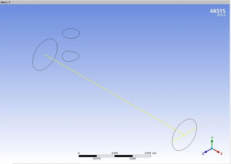
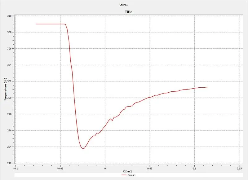
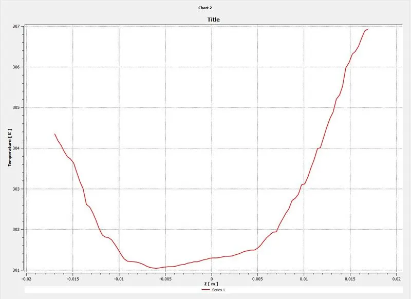
Temperature line plots along and across the length of the pipe:
Temperature plot along the length of pipe:
Temperature plot across the length of pipe:
2-b: Short mixing tee (momentum ratio: 4).
Geometry and Meshing were the same as case 2-a.
Setup:
Checking of mesh is done. Steady-state, pressure-based, and absolute velocity formation solver is used. Energy is selected because measuring temperature is involved.
The models selected: K-epsilon realizable.
Materials are selected. Cell zones and the same boundary conditions are given for both models.
Boundary conditions:
Inlet-x: Type-velocity inlet: Velocity of air= 3 m/s and Temperature of air= 309 K.
`Momentum ratio=(velocity of cold air)/(velocity of hot air)`
Taken momentum ratio =4. So the velocity of cold air is 12 m/s.
Inlet-y: Type-velocity inlet: Velocity of air= 12 m/s and Temperature of air= 292 K.
Outlet: Type-pressure outlet.
Definitions: Area weighted average and Standard deviation for temperature are plotted.
Initialization: Hybrid
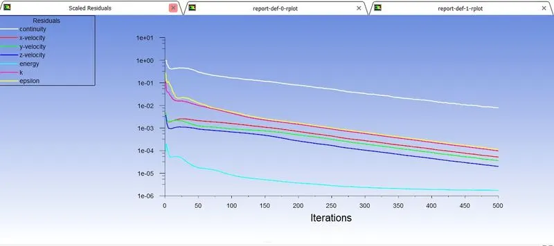
The number of iterations: 500.
Results:
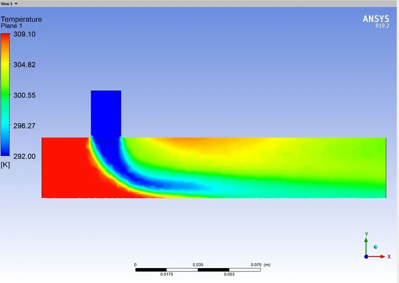
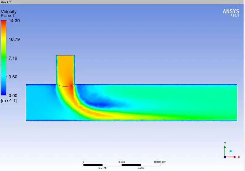
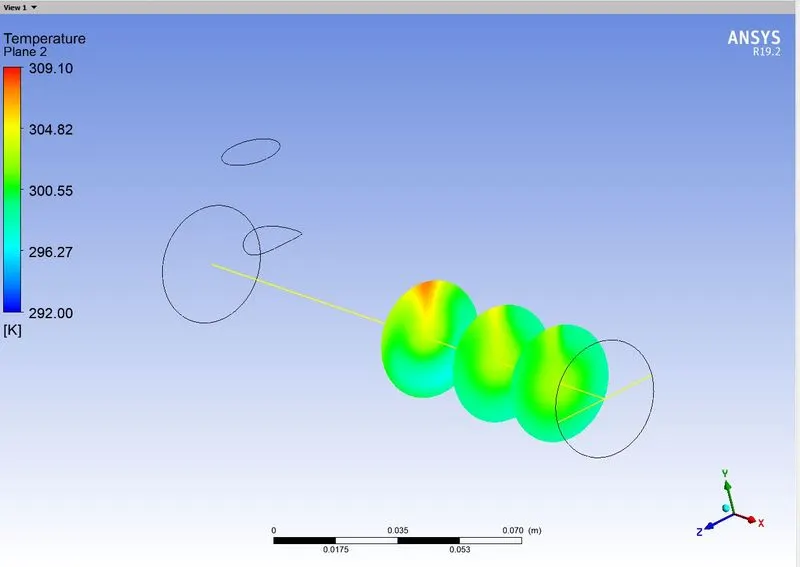
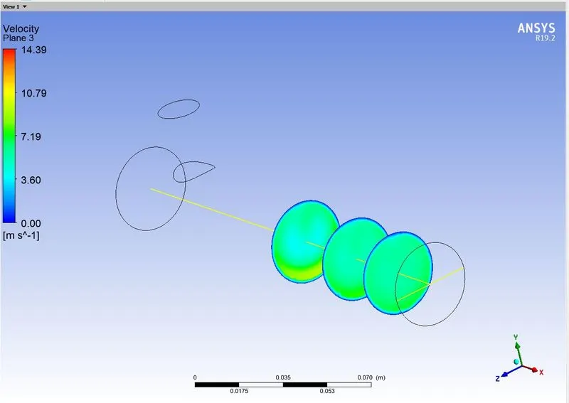
Temperature and velocity contours:
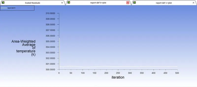
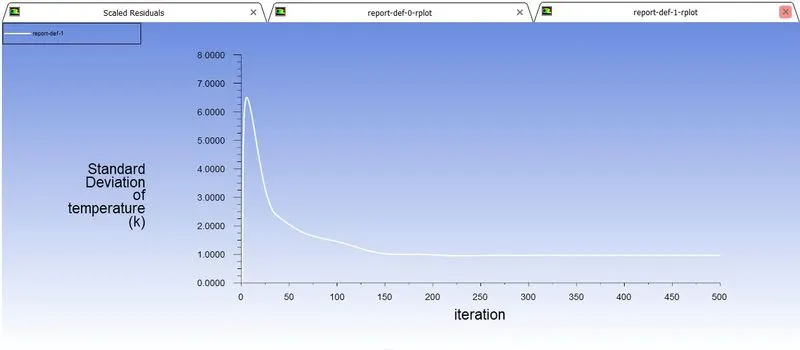
Residual plot, and Area-weighted average and standard deviation of temperature plots:
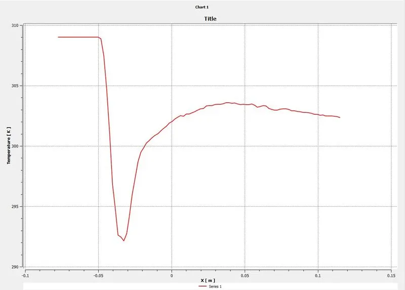
Temperature plot along the length of pipe:
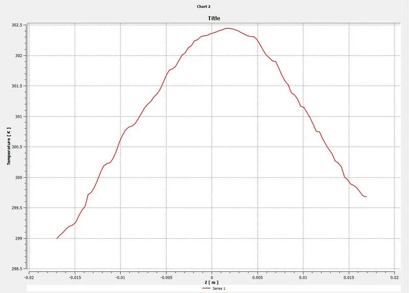
Temperature plot across the length of pipe:
2-c: Long mixing tee (momentum ratio: 2).
Geometry:
Loading up the geometry and volume extraction for the geometry is done using Ansys Spaceclaim in the Fluent module of the Ansys Workbench.
Meshing:
Meshing is done in Ansys workbench meshing in the fluent module. Element size of 0.002 m is used. Also named selections: Inlet-x, Inlet-y, Outlet, and Walls are given.
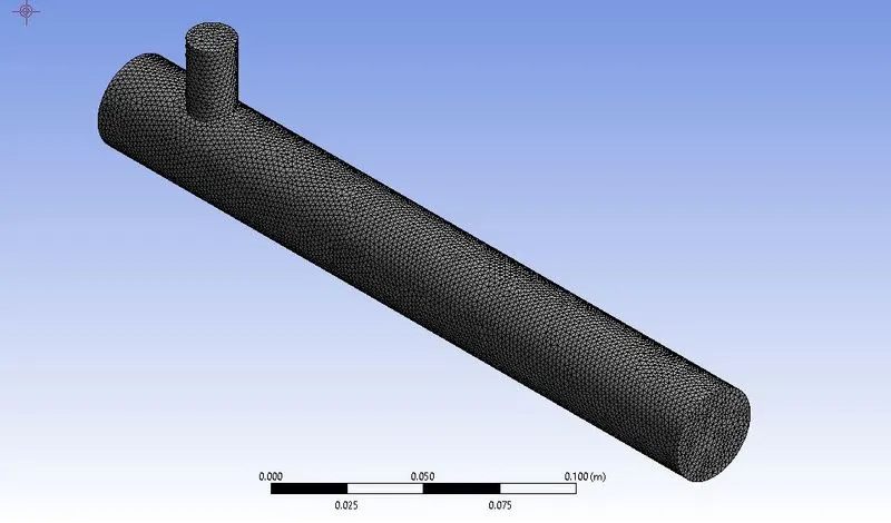
The number of elements: 141714.
Setup:
Checking of mesh is done. Steady-state, pressure-based, and absolute velocity formation solver is used. Energy is selected because measuring temperature is involved.
The models selected: K-epsilon realizable.
Materials are selected. Cell zones and the same boundary conditions are given for both models.
Boundary conditions:
Inlet-x: Type-velocity inlet: Velocity of air= 3 m/s and Temperature of air= 309 K.
`Momentum ratio=(velocity of cold air)/(velocity of hot air)`
Taken momentum ratio =2. So the velocity of cold air is 6 m/s.
Inlet-y: Type-velocity inlet: Velocity of air= 6 m/s and Temperature of air= 292 K.
Outlet: Type-pressure outlet.
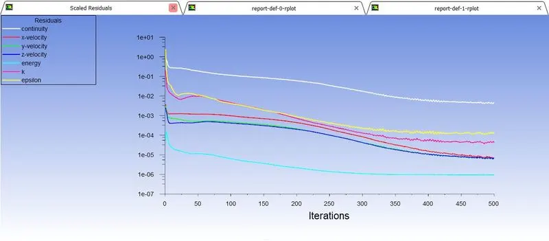
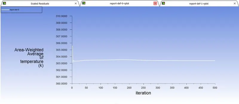
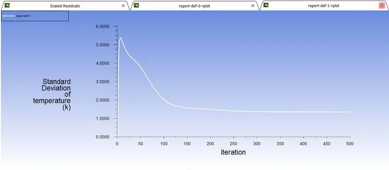
Definitions: Area weighted average and Standard deviation for temperature are plotted.
Initialization: Hybrid
The number of iterations: 500.
Results:
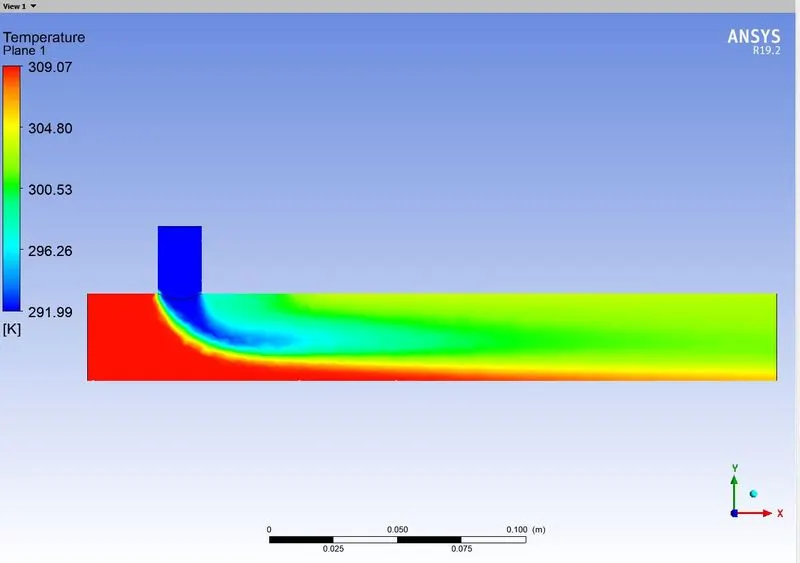
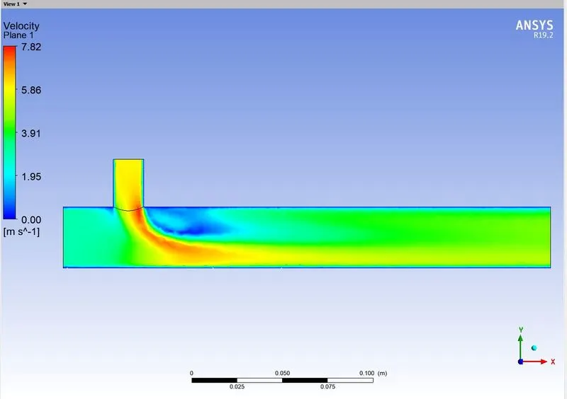
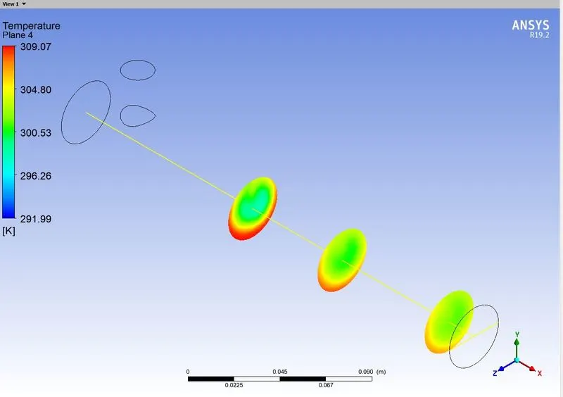
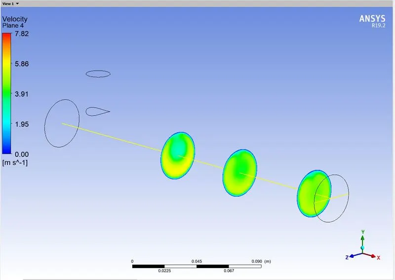
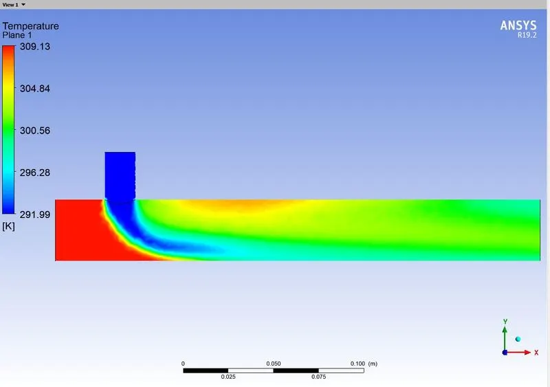
Temperature and velocity contours:
Residual plot, and Area-weighted average and standard deviation of temperature plots:
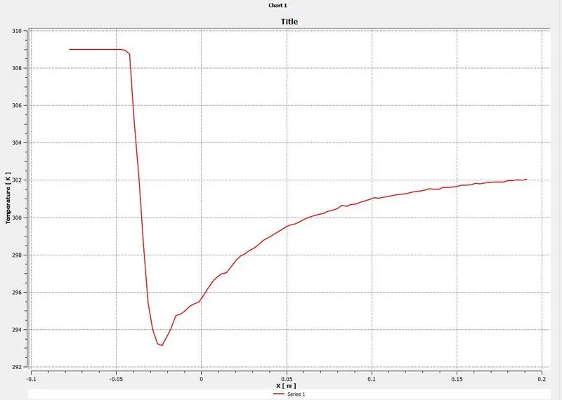
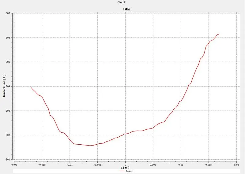
Temperature line plots along and across the length of the pipe:
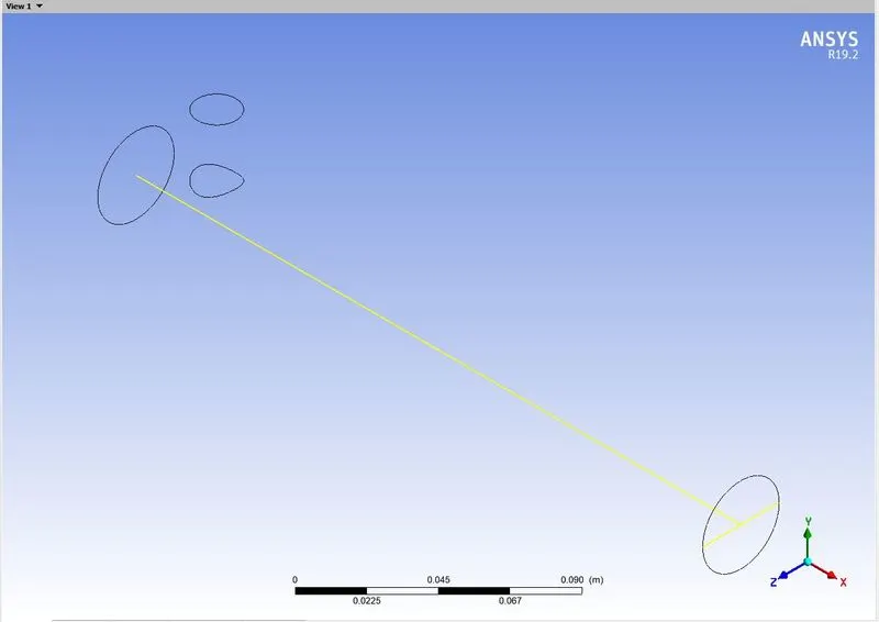
Temperature line plots along the length of the pipe:
Temperature line plots across the length of the pipe:
2-d: Long mixing tee (momentum ratio: 4).
Geometry and Meshing were the same as case 2-c.
Setup:
Checking of mesh is done. Steady-state, pressure-based, and absolute velocity formation solver is used. Energy is selected because measuring temperature is involved.
The models selected: K-epsilon realizable.
Materials are selected. Cell zones and the same boundary conditions are given for both models.
Boundary conditions:
Inlet-x: Type-velocity inlet: Velocity of air= 3 m/s and Temperature of air= 309 K.
`Momentum ratio=(velocity of cold air)/(velocity of hot air)`
Taken momentum ratio =4. So the velocity of cold air is 12 m/s.
Inlet-y: Type-velocity inlet: Velocity of air= 12 m/s and Temperature of air= 292 K.
Outlet: Type-pressure outlet.
Definitions: Area weighted average and Standard deviation for temperature are plotted.
Initialization: Hybrid
The number of iterations: 500.
Results:
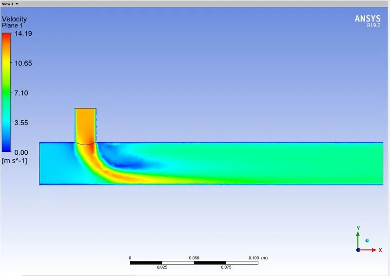
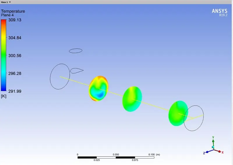
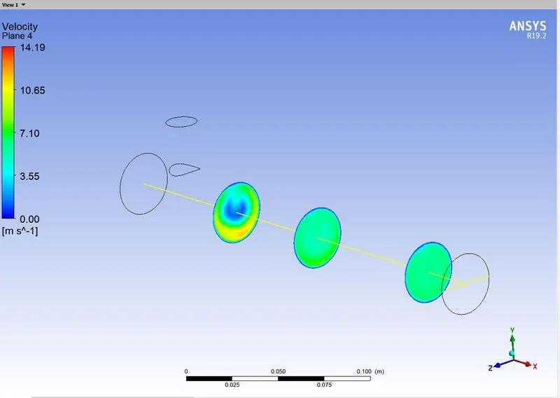
Temperature and velocity contours:
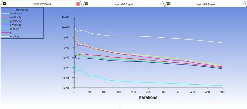
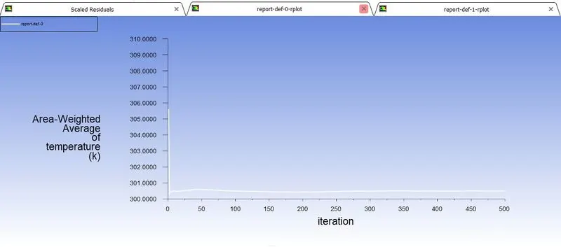
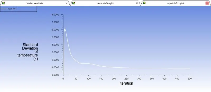
Residual plot, and Area-weighted average and standard deviation of temperature plots:
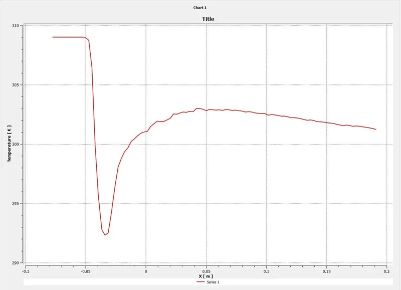
Temperature line plots along the length of the pipe:
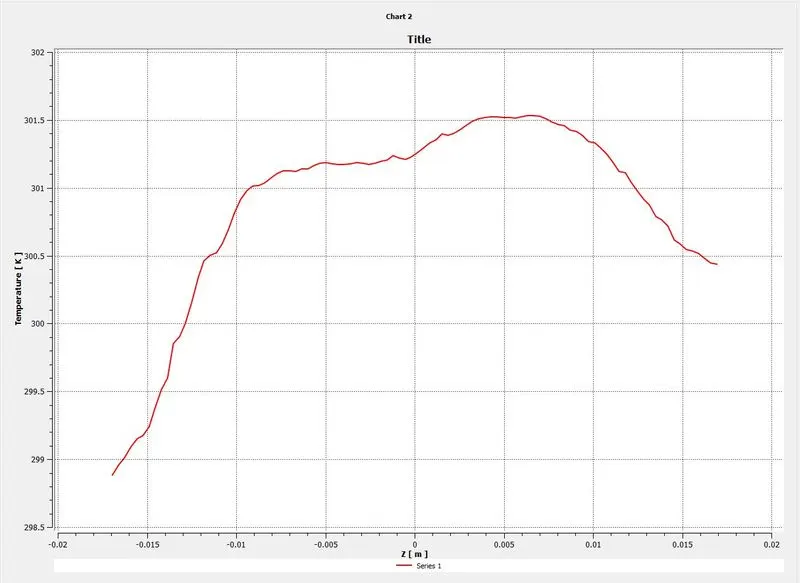
Temperature line plots across the length of the pipe:
Observations:

Case 2-d: Long mixing tee of momentum ratio:4 produced the best result of average outlet temperature at 300.50 K with the next best result being Case 2-b: Short mixing tee of momentum ratio:4 with average outlet temperature at 300.55 K. Here the effect of length and momentum ratio play a crucial role. The high velocity of flow is shown to be effective to get lower average outlet temperature and better mixing at the outlet. Therefore, a higher momentum ratio is necessary. In the temperature contour of long tee cases, the high temperatures flow thoroughly mixes with the rest of the flow. As the Length of the mixing tee increases, because of diffusion, flow always gives slightly better mixing of two-fluid and will have time to mix.
Recommend model is the long tee model with the high-velocity inlet for application. This is because we have the best result of average outlet temperature at 300.50 K and also show comparatively low standard deviation in the case of long tee compared to the short tee for both momentum ratios.
3. Grid Independence Test:
A Mesh independence study is being performed on the Short tee with a momentum ratio of 2.
Results:

Conclusions:
Simulated hot and cold airflow in mixing tee of varying in length: short and long through their inlets at different velocities with momentum ratios 2 and 4. Tested K-Epsilon and K-Omega models with short mixing tee with momentum ratio 2 which resulted in K-epsilon being the suitable model. Velocity and temperature contour plots on the cut planes along and across the pipe and line plots along and across the length of the pipe were presented for each case. Long mixing tee with momentum ratio of 4 showed the best result with the temperature at outlet being 300.50 K and also showing comparatively low stand deviation in temperature. Discussed the effect of length and momentum ratio on results. Perform Mesh independent study for any one case.