Week 5 - Mid term project - Solving the steady and unsteady 2D heat conduction problem
Objective: Solving the steady and unsteady 2 - Dimensional heat conduction problem using explicit and implicit scheme methods.
1. Solving 2 - Dimensional steady heat conduction problem using explicit scheme.
2-D steady heat conduction equation is as follows : `((del^2T)/(delx^2) + (del^2T)/(dely^2)) = 0`
we discretize the equation using central difference scheme.
`((del^2T)/(delx^2) ) = (T(i+1,j) - 2*T(i,j) + T(i-1,j))/(Deltax^2)`
`((del^2T)/(dely^2) ) = (T(i,j+1) - 2*T(i,j) + T(i,j-1))/(Deltay^2)`
Assuming `Deltax^2 = Deltay^2`, The final equation is
`T(i,j) = (1/4)*(T(i+1,j) + T(i-1,j)) + T(i,j+1) + T(i,j-1))`
Jacobi method:
`T(i,j) = (1/4)*(T_(old)(i+1,j) + T_(old)(i-1,j)) + T_(old)(i,j+1) + T_(old)(i,j-1))`
Gauss Seidal:
`T(i,j) = (1/4)*(T_(old)(i+1,j) + T(i-1,j)) + T_(old)(i,j+1) + T(i,j-1))`
SOR:
`T(i,j) = ((1-alpha)*T_(old)(i,j)+ (alpha*0.25)*(T(i-1,j) + T(i,j+1) + T(i,j-1)))`
The code for solving is given below :
%2-D steady state heat conduction equation is (D^2T/dx^2 + D^2T/dy^2)

clear all
clc

L = 1;
nx = 20;
ny = nx; %taking same grid points for nx and ny
x = linspace(0,L,nx);
y = linspace(0,L,ny);
dx = x(2) - x(1);
dy = y(2) - y(1);
error = 9e9;
tol = 1e-4;
T = ones(nx,ny);

%Boundary conditions

T_Top = 600; T_Bottom = 900; T_Left = 400; T_Right = 800;
T(2:ny-1,1) = T_Left;
T(2:ny-1,nx) = T_Right;
T(1,2:nx-1) = T_Top;
T(nx,2:ny-1) = T_Bottom;

%For Corner points temperatures, taking average

T(1,1) = (T_Top + T_Left)/2;
T(1,ny) = (T_Top + T_Right)/2;
T(nx,1) = (T_Bottom + T_Left)/2;
T(nx,ny) = (T_Bottom + T_Right)/2;

iterative_solver = 1; %input for methods. enter manually for each method

if iterative_solver ==1
jacobi_method( T, error, tol, nx, ny,x,y)

elseif iterative_solver ==2
    gauss_method( T, error, tol, nx, ny,x,y)

elseif iterative_solver ==3
    SOR_method( T, error, tol, nx, ny,x,y)
end

%creating a function to access Jacobi Method

function jacobi_method( T, error, tol, nx, ny,x,y)
[X,Y] = meshgrid(x,y);
T_old = T;
jacobi_iter = 1;

while(error>tol)

    for i=2:nx-1

        for j=2:ny-1

            T(i,j) = 0.25*(T_old(i+1,j)+T_old(i-1,j)+T_old(i,j+1)+T_old(i,j-1));

        end

    end
        error = max(max(abs(T_old - T)));
        T_old = T;
        jacobi_iter = jacobi_iter + 1;

end

    %plotting
    figure(1)
    contourf(x,y,T);
    clabel(contourf(x,y,T));
    colorbar
    colormap(jet)
    xlabel('x axis')
    ylabel('y axis')
    title_text = sprintf('iteration number = %d',jacobi_iter);
    title(title_text)
    set(gca, 'ydir' , 'reverse' )

end

%Creating a function to access Gauss siedal method

function gauss_method( T, error, tol, nx, ny,x,y)
[X,Y] = meshgrid(x,y);
T_old = T;
gauss_iter = 1;

while(error>tol)

    for i=2:nx-1

        for j=2:ny-1

            T(i,j) = 0.25*(T_old(i+1,j)+T(i-1,j)+T_old(i,j+1)+T(i,j-1));

        end

    end
        error = max(max(abs(T_old - T)));
        T_old = T;
        gauss_iter = gauss_iter + 1;

end

   %plotting
    figure(1)
    contourf(x,y,T);
    clabel(contourf(x,y,T));
    colorbar
    colormap(jet)
    xlabel('x axis')
    ylabel('y axis')
    title_text = sprintf('iteration number = %d',gauss_iter);
    title(title_text)
    set(gca, 'ydir' , 'reverse' )

end

%Creating a function to access SOR method

function SOR_method( T, error, tol, nx, ny,x,y)
[X,Y] = meshgrid(x,y);
T_old = T;
alpha = 1.5;
SOR_iter = 1;

while(error>tol)

    for i=2:nx-1

        for j=2:ny-1

            T(i,j) = ((1-alpha)*T_old(i,j) + (alpha*0.25*(T_old(i+1,j)+T(i-1,j)+T_old(i,j+1)+T(i,j-1))));

        end

    end
        error = max(max(abs(T_old - T)));
        T_old = T;
        SOR_iter = SOR_iter + 1;

end

    %plotting
    figure(1)
    contourf(x,y,T);
    clabel(contourf(x,y,T));
    colorbar
    colormap(jet)
    xlabel('x axis')
    ylabel('y axis')
    title_text = sprintf('iteration number = %d',SOR_iter);
    title(title_text)
    set(gca, 'ydir' , 'reverse' )

end
The results are as follows :
1. Solved using Jacobi Method of iteration
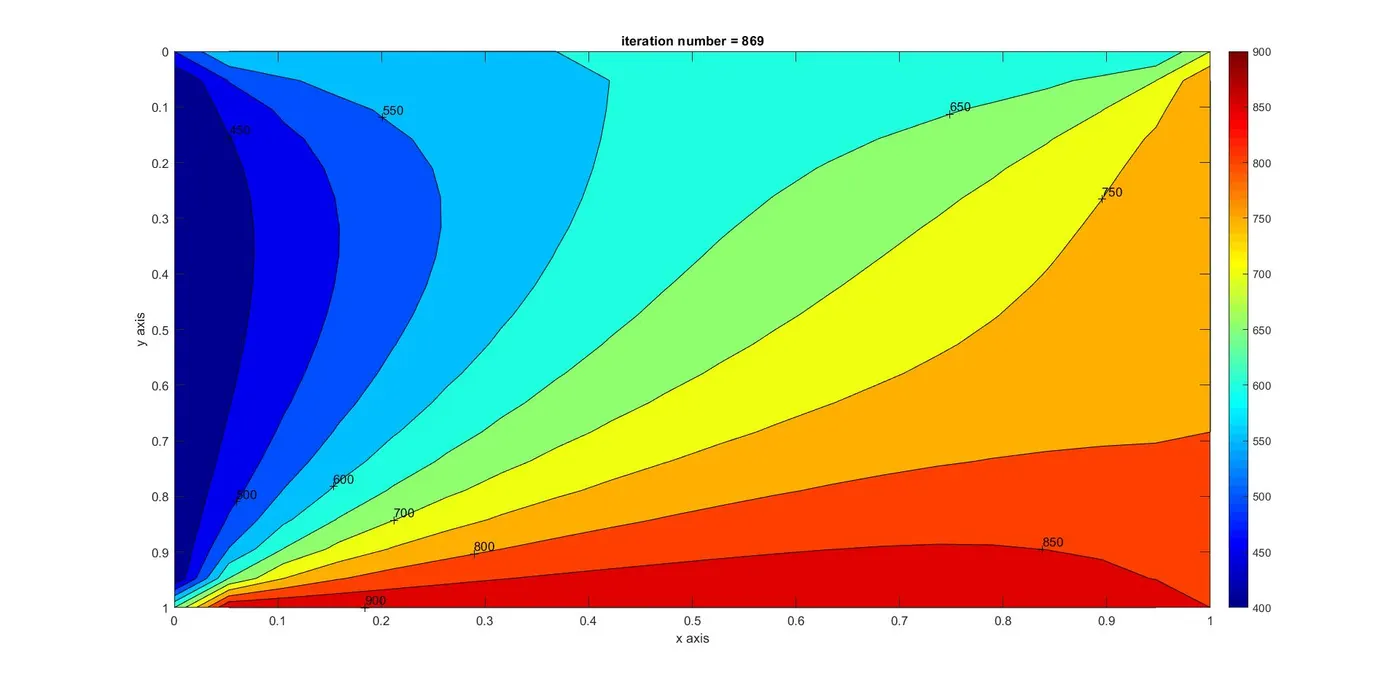
The number of iterations taken = 869
2. Solved using Gauss Seidel method of iteration
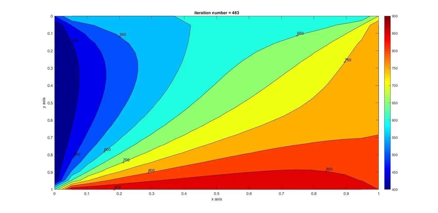
The number of iterations taken = 463
3. Solved using SOR method of iteration
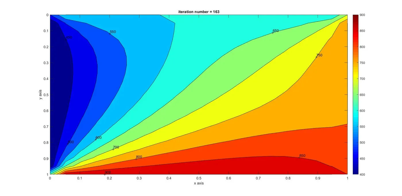
The number of iterations taken = 163
For solving 2-D steady heat conduction equation explicitly, Successive Relaxation is more preferred as it is taking less iterations and computational space and time.
2. Solving 2 - Dimensional unsteady/transient heat conduction problem using explicit scheme.
2-D steady heat conduction equation is as follows : `(delT)/(delt) = alpha*((del^2T)/(delx^2) + (del^2T)/(dely^2))`
Discretization is as follows :
`((del^2T)/(delx^2) ) = (T^n(i+1,j) - 2*T^n(i,j) + T^n(i-1,j))/(Deltax^2)`
`((del^2T)/(dely^2) ) = (T^n(i,j+1) - 2*T^n(i,j) + T^n(i,j-1))/(Deltay^2)`
`(delT)/(delt) = (T^(n+1)(i,j) -T^n(i,j))/(Deltat)`
Let `k1 = (alpha*DeltaT)/(Deltax^2)`
`k2 = (alpha*DeltaT)/(Deltay^2)`
Assuming `Deltax^2 = Deltay^2`, The final equation is
`T^(n+1)(i,j) = T^n(i,j) + k1*(T^n(i+1,j) + T^n(i-1,j) -2*T^n(i,j)) +k2*(T^n(i,j+1) + T^n(i,j-1) -2*T^n(i,j))`
The code for solving is given below :
clear all
clc

L = 1;
nx = 20;
ny = nx; %taking same grid points for nx and ny
x = linspace(0,L,nx);
y = linspace(0,L,ny);
dx = x(2) - x(1);
dy = y(2) - y(1);
DT = 0.001;
nt = 1000;
alpha = 1.172e-5;
k1 = (alpha*DT)/dx^2;
k2 =  (alpha*DT)/dy^2;
error = 9e9;
tol = 1e-4;
T = ones(nx,ny);

%Boundary conditions

T_Top = 600; T_Bottom = 900; T_Left = 400; T_Right = 800;
T(2:ny-1,1) = T_Left;
T(2:ny-1,nx) = T_Right;
T(1,2:nx-1) = T_Top;
T(nx,2:ny-1) = T_Bottom;

%For Corner points temperatures, taking average

T(1,1) = (T_Top + T_Left)/2;
T(1,ny) = (T_Top + T_Right)/2;
T(nx,1) = (T_Bottom + T_Left)/2;
T(nx,ny) = (T_Bottom + T_Right)/2;

iterative_solver =1;%enter manually for each iteration method

if iterative_solver ==1
jacobi_tran_exp( T, error, tol, nx, ny,x,y,k1,k2,nt)
end

%creating a function to access

function jacobi_tran_exp( T, error, tol, nx, ny,x,y,k1,k2,nt)
[X,Y] = meshgrid(x,y);
T_old = T;
jacobi_iter = 1;

for k=1:nt

    %while(error>tol)

        for i=2:nx-1

            for j=2:ny-1
                term1 = T_old(i,j);
                term2 = k1*(T_old(i+1,j) + T_old(i-1,j) - 2*(T_old(i,j)));
                term3 = k2*(T_old(i,j+1) + T_old(i,j-1) - 2*(T_old(i,j)));
                T(i,j) = term1+term2+term3;
            end

        end
        error = max(max(abs(T_old - T)));
        T_old = T;
        jacobi_iter = jacobi_iter + 1;
    %end

end
    %plotting
    figure(1)
    contourf(x,y,T);
    clabel(contourf(x,y,T));
    colorbar
    colormap(jet)
    xlabel('x axis')
    ylabel('y axis')
    title_text = sprintf('iteration number = %d',jacobi_iter);
    title(title_text)
    set(gca, 'ydir' , 'reverse' )
end
The results are as follows :
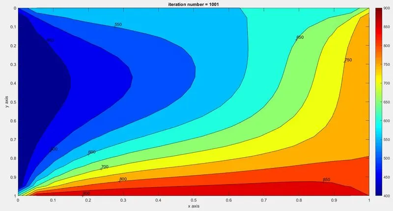
The number of iterations taken = 1001
3. Solving 2 - Dimensional unsteady/transient heat conduction problem using implicit scheme.
2-D steady heat conduction equation is as follows : `(delT)/(delt) = alpha*((del^2T)/(delx^2) + (del^2T)/(dely^2))`
Discretization is as follows :
`((del^2T)/(delx^2) ) = (T^(n+1)(i+1,j) - 2*T^(n+1)(i,j) + T^(n+1)(i-1,j))/(Deltax^2)`
`((del^2T)/(dely^2) ) = (T^(n+1)(i,j+1) - 2*T^(n+1)(i,j) + T^(n+1)(i,j-1))/(Deltay^2)`
`(delT)/(delt) = (T^(n+1)(i,j) -T^n(i,j))/(Deltat)`
Let `k1 = (alpha*DeltaT)/(Deltax^2)`
`k2 = (alpha*DeltaT)/(Deltay^2)`
Assuming `Deltax^2 = Deltay^2`, The final equation is
`T^(n+1)(i,j) = 1/(1 + 2k1 + 2k2) * (T^n(i,j) + (k1*(T^(n+1)(i+1,j) + T^(n+1)(i-1,j)) +k2*(T^(n+1)(i,j+1) + T^(n+1)(i,j-1)))`
The code for solving is given below :
clear all
clc

L = 1;
nx = 20;
ny = nx; %taking same grid points for nx and ny
x = linspace(0,L,nx);
y = linspace(0,L,ny);
dx = x(2) - x(1);
dy = y(2) - y(1);
DT = 1;
nt = 100000;
alpha = 1.172e-5;
k1 = (alpha*DT)/dx^2;
k2 =  (alpha*DT)/dy^2;
error = 9e9;
tol = 1e-4;
T = ones(nx,ny);

%Boundary conditions

T_Top = 600; T_Bottom = 900; T_Left = 400; T_Right = 800;
T(2:ny-1,1) = T_Left;
T(2:ny-1,nx) = T_Right;
T(1,2:nx-1) = T_Top;
T(nx,2:ny-1) = T_Bottom;

%For Corner points temperatures, taking average

T(1,1) = (T_Top + T_Left)/2;
T(1,ny) = (T_Top + T_Right)/2;
T(nx,1) = (T_Bottom + T_Left)/2;
T(nx,ny) = (T_Bottom + T_Right)/2;

iterative_solver =1;%enter manually for each method

if iterative_solver ==1
    jacobi_tran_imp( T, error, tol, nx, ny, x, y, k1, k2, nt)
elseif iterative_solver ==2
    gauss_tran_imp( T, error, tol, nx, ny, x, y, k1, k2, nt)
elseif iterative_solver ==3
    SOR_tran_imp( T, error, tol, nx, ny, x, y, k1, k2, nt)
end

%Creating function to access Jacobi method

function jacobi_tran_imp( T, error, tol, nx, ny, x, y, k1, k2, nt)

[X,Y] = meshgrid(x,y);
T_old = T; %for jacobi and gauss
T_prev = T_old; %for implicit scheme creating a copy of T_old
jacobi_iter = 1;
term1 = (1 + (2*k1) + (2*k2))^(-1);
term2 = k1*term1;
term3 = k2*term1;

for k=1:nt

    while(error>tol)

        for i=2:nx-1

            for j=2:ny-1

                H = (T_old(i+1,j) + T_old(i-1,j));
                V = (T_old(i,j+1) + T_old(i,j-1));
                T(i,j) = ((T_prev(i,j)*term1) + (H*term2) + (V*term3));

            end

        end

        error = max(max(abs(T_old - T)));
        T_old = T;
        jacobi_iter = jacobi_iter + 1;


    end
    error =1;
    T_prev = T;
end

    %plotting
    figure(1)
    contourf(x,y,T);
    clabel(contourf(x,y,T));
    colorbar
    colormap(jet)
    xlabel('x axis')
    ylabel('y axis')
    title_text = sprintf('iteration number = %d',jacobi_iter);
    title(title_text)
    set(gca, 'ydir' , 'reverse' )
end

%Creating function to access Gauss method

function gauss_tran_imp( T, error, tol, nx, ny, x, y, k1, k2, nt)
[X,Y] = meshgrid(x,y);
T_old = T; %for jacobi and gauss
T_prev = T_old; %for implicit scheme creating a copy of T_old
gauss_iter = 1;
term1 = (1 + (2*k1) + (2*k2))^(-1);
term2 = k1*term1;
term3 = k2*term1;

for k=1:nt

    while(error>tol)

        for i=2:nx-1

            for j=2:ny-1

                H = (T_old(i+1,j) + T(i-1,j));
                V = (T_old(i,j+1) + T(i,j-1));
                T(i,j) = ((T_prev(i,j)*term1) + (H*term2) + (V*term3));

            end

        end

        error = max(max(abs(T_old - T)));
        T_old = T;
        gauss_iter = gauss_iter + 1;


    end
    error =1;
    T_prev = T;

end

    %plotting
    figure(1)
    contourf(x,y,T);
    clabel(contourf(x,y,T));
    colorbar
    colormap(jet)
    xlabel('x axis')
    ylabel('y axis')
    title_text = sprintf('iteration number = %d',gauss_iter);
    title(title_text)
    set(gca, 'ydir' , 'reverse' )
end

%Creating function for SOR method

function SOR_tran_imp( T, error, tol, nx, ny, x, y, k1, k2, nt)
[X,Y] = meshgrid(x,y);
T_old = T; %for jacobi and gauss
T_prev = T_old; %for implicit scheme creating a copy of T_old
alpha = 1.01;
SOR_iter = 1;
term1 = (1 + (2*k1) + (2*k2))^(-1);
term2 = k1*term1;
term3 = k2*term1;

for k=1:nt

    while(error>tol)

        for i=2:nx-1

            for j=2:ny-1

                H = (T_old(i+1,j) + T(i-1,j));
                V = (T_old(i,j+1) + T(i,j-1));
                Z = ((T_prev(i,j)*term1) + (H*term2) + (V*term3));
                T(i,j) = ((T_old(i,j))*(1-alpha)) + (alpha*Z);

            end

        end

        error = max(max(abs(T_old - T)));
        T_old = T;
        SOR_iter = SOR_iter + 1;


    end
    error =1;
    T_prev = T;

end

    %plotting
    figure(1)
    contourf(x,y,T);
    clabel(contourf(x,y,T));
    colorbar
    colormap(jet)
    xlabel('x axis')
    ylabel('y axis')
    title_text = sprintf('iteration number = %d',SOR_iter);
    title(title_text)
    set(gca, 'ydir' , 'reverse' )
end
The results are as follows :
1. Solved using Jacobi Method of iteration
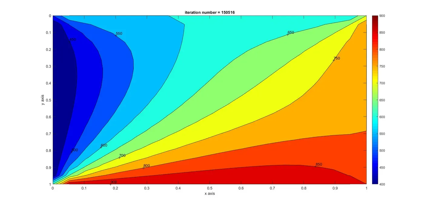
The number of iterations taken = 150516
2. Solved using Gauss Seidel method of iteration
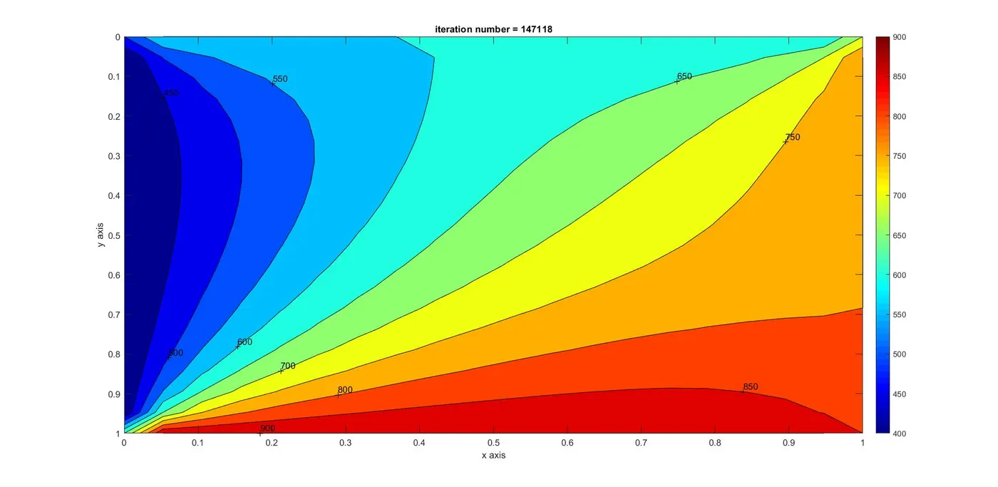
The number of iterations taken = 147118
3. Solved using SOR method of iteration
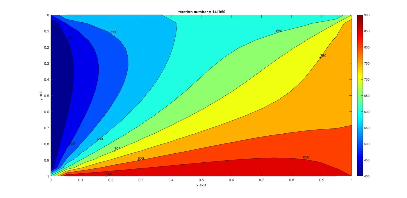
The number of iterations taken = 141050
For solving 2-D unsteady heat conduction equation implicitly, Successive Relaxation is more preferred as it is taking less iterations and computational space and time.
4. Result Discussion :
For solving 2 - Dimensional steady heat conduction problem using explicit scheme, Successive Over Realxation method proved to be more efficient as it took less iterations to solve while compared to Jacobi and Gauss-Seidel methods respectively with lesser error.
For solving 2 - Dimensional unsteady/transient heat conduction problem using implicit scheme, Successive Over Realxation method proved to be more efficient as it took less iterations to solve while compared to Jacobi and Gauss-Seidel methods respectively with lesser error.
Also Steady state equation required less time to solve using iteration methods than the unsteady/transient equation.