Week 2 - Flow over a Cylinder.

AIM :

To simulate the flow over a cylinder and capture the Von Karman vortices formed behind the cylinder to the direction of flow in steady and transient state for various Reynolds number and also to calculate the strouhal number when the Reynolds number is 100.

OBJECTIVE :

• To create the 2D cylinderal surface and its fluid domain using spaceclaim in Ansys fluent.
• To perform meshing with triangular mesh elements and create inflation layer to the surface of the cylinder.
• To create a moniter point for finding the velocity behind the cylinder after the simulation.
• To setup the domain for simulation and analyse the formation of Von Karman vortices for different cases which have different Reynolds numbers, which is done by varying the only the velocity of the fluid for each case.
• To create various plots for co-efficient of drag, lift and vertex velocity at the monitor point and also to create velocity and pressure contour plots in post processing.
• To calculate the Strouhal Number for Re= 100 for both steady and transient state.

INTRODUCTION :

In this project, we are going to simulate the flow over a cylinder inorder to capture the vortex shedding that is formed behind the cylinder surface. This is done for various cases by varying the velocity of the fluid flow for each case inorder to change the reynolds number and so by taking the user defined fluid with constant density of 1 kg/m^3 and viscosity of 0.05 kg/m-s. This simulation is done with steady state and transient state for Reynolds number is 100 and so as to analyse the vortex formation for both the cases and also to calculate the Strouhal number.

Karman vortex street:

It is repeating pattern of swirling vortices caused by a process known as vortex shedding which is responsible for the unsteady seperation of flow of a fluid.

Strouhal Number :

It is a dimensionless number used in studying the vibrations of a body past which is flowing. It is equal to characteristic dimension of the body times the frequency of vibrations divided by the fluid velocity relative to the body.

• `Sr = omega * D / V`

Where,

• `omega` is the frequency (in Hz)
• D is the diameter (in meters)
• V is the velocity (m/s)

Reynolds number :

It is a dimensionless quantity that is used to determine the type of flow pattern as laminar or turbulent while flowing through a pipe. Reynolds number is defined by the ratio of inertial forces to that of viscous forces.

• Reynolds number = inertial force / viscous force
• `R_e = rho * V * D / mu`

Where,

• R_e is the Reynolds number
• ρ is the density of the fluid
• V is the velocity of flow
• D is the pipe diameter
• μ is the viscosity of the fluid

In this problem to simulate the flow over a cylinder for different Reynolds number values, we vary only the velocity of the fluid for every case since it is directly proportional to Reynolds number and this is also done by keeping the viscosity of the fluid as 0.05 kg/m-s and density as 1 kg / m^3 and diameter of the cylinder as given ( = 2m).

• For internal fluid flow, If Reynolds number < 2400, it is a laminar flow.
• For internal fluid flow, If Reynolds number > 2400, it is a turbulent flow.
• For external fluid flow, If Reynolds number < 2*10^5, it is laminar flow.
• For external fluid flow, If Reynolds number > 5*10^5, it is a turbulent flow.

`V = R_e * mu /( rho * D)`

PROBLEM SETUP :

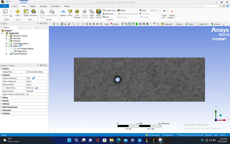
The mesh element size is taken as 500 mm for all the cases since it is a optimum element size for finding the accurate results in less computational time.

1. For Re = 10, V = 0.25 m/s
2. For Re = 100, V = 2.5 m/s
3. For Re = 1000, V = 25 m/s
4. For Re = 10000, V = 250 m/s
5. For Re = 100000, V = 2500 m/s

The simulation is done for steady as well as transient state condition,

• The steady state is the state that is established after a certain time in your system.
• The transient state is basically between the beginning of the event and the steady state.

PROCEDURE :

1. For Reynolds number = 10 (i.e,velocity = 0.25 m/s) Steady state :

PRE-PROCESSING :

• Open spaceclaim from the Fluid Flow (Fluent) analysis system in Ansys workbench and In spaceclaim, change the sketch plane to XY using the sketch plane option.

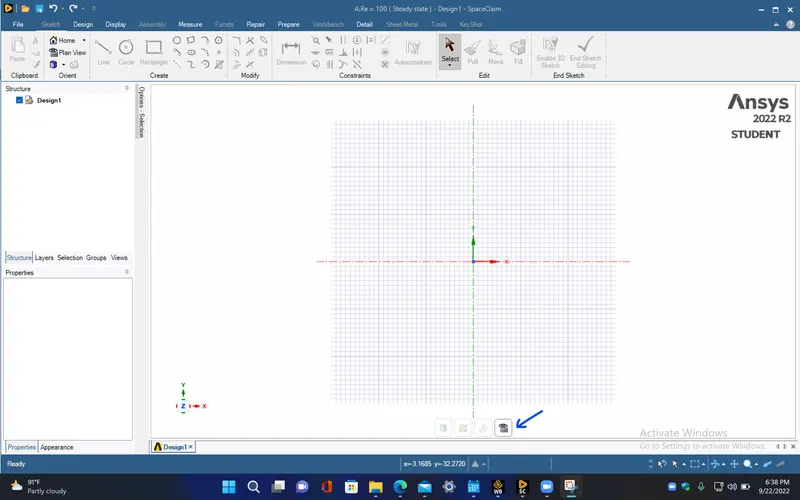
• To create a cylindrical surface, create a circle with the diameter of 2 meters from the XY origin and create a rectangular fluid domain with the respective distances (At front - 10*diameter of cylinder = 20m , At back - 20*diameter = 40m, At top and bottom - 5*diameter = 10m for each) from the centre of the circle.

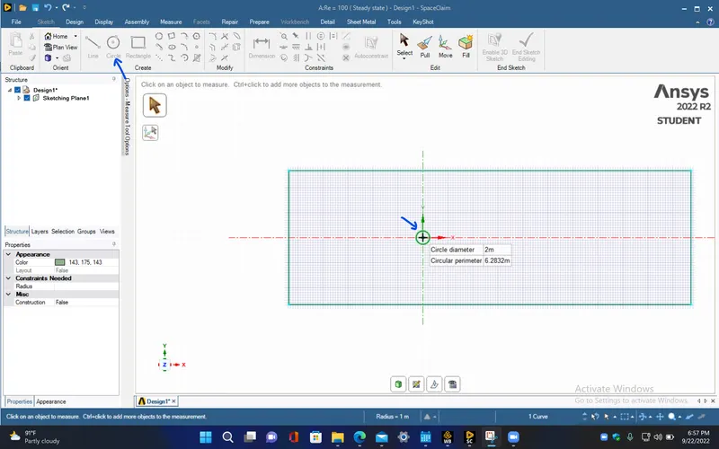
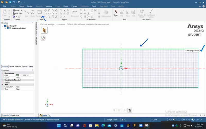
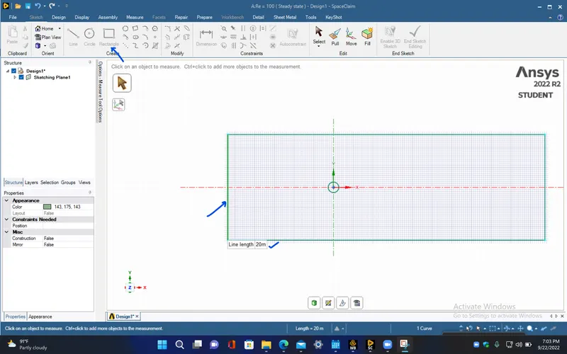
• To convert the 1D geometry into a 2D surface, use the pull option under sketch.

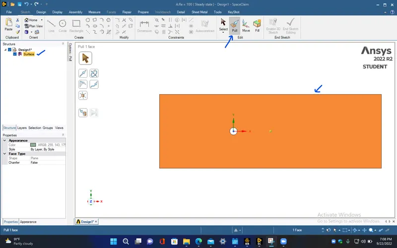
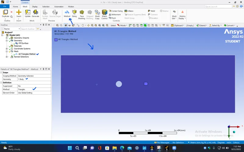
• Now, close the spaceclaim window and open mesh window, To change the mesh elements to triangular shape, click new method option under mesh, select the surface and change it to traingle.

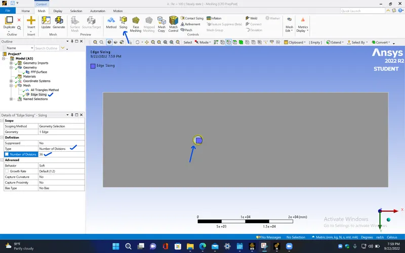
• To capture the cylindrical surface properly inorder to get the accurate results during simulation, use sizing option under mesh, select the circular edge and give the number of division as 36 which will divide the circumference of the circle with 36 equal parts.

• Now, generate mesh with mesh element size as 500mm which will be the optimum length for this simulation.

• Now, insert inflation layers near to the cylindrical edge by seleting the edge and giving the first layer thickness as 5mm, number of layers as 6 in growth rate of 1.2. This will capture the geometry near the cylindrical surface more accurately and will give more accurate results during simulation.

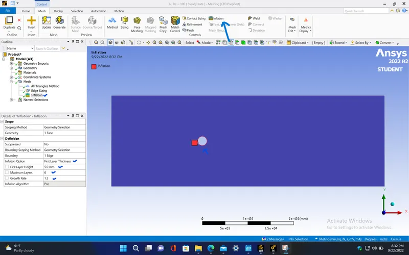
• Now, update the mesh.

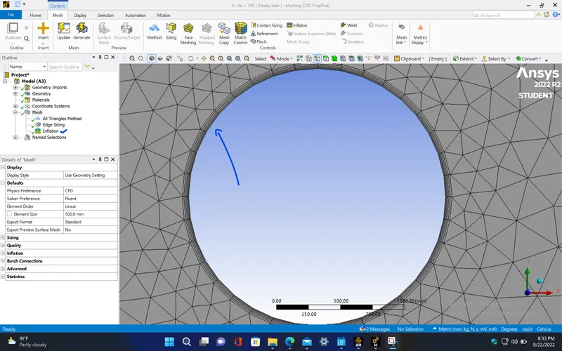
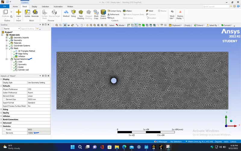
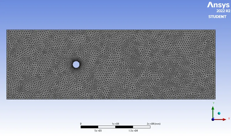
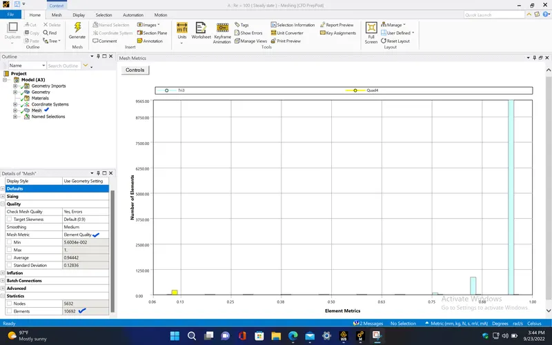
Cells	Faces	Nodes
10692	16324	5632

SETUP AND SOLVING :

• Open setup window and give the following parameters

Model	Settings
Space	2D

Model	Settings
Time	Steady
Viscous	Laminar

FLUID PROPERTIES :

Fluid	user-defined-fluid
Density	1 kg/m^3
Cp (Specific Heat)	1006.43 J/(kg K)
Thermal Conductivity	0.0242 W/(m K)
Viscosity	0.05 kg/(m s)
Molecular Weight	28.966 kg/kmol

BOUNDARY CONDITIONS :

inlet
Velocity Specification Method	Magnitude, Normal to Boundary
Reference Frame	Absolute
Velocity Magnitude [m/s]	0.25
Supersonic/Initial Gauge Pressure [Pa]	0
outlet
Backflow Reference Frame	Absolute
Gauge Pressure [Pa]	0
Backflow Direction Specification Method	Normal to Boundary

Symmetry
symmetry	symmetry
cylinder_wall
Wall Motion	Stationary Wall
Shear Boundary Condition	No Slip

REFERENCE VALUES :

Area	2 m^2
Density	1 kg/m^3
Depth	1 m
Enthalpy	0 J/kg
Length	2 m
Pressure	0 Pa
Temperature	288.16 K
Velocity	0.25 m/s
Viscosity	0.05 kg/(m s)
Ratio of Specific Heats	1.4
Yplus for Heat Tran. Coef.	300
Reference Zone	fff_surface

SOLVER :

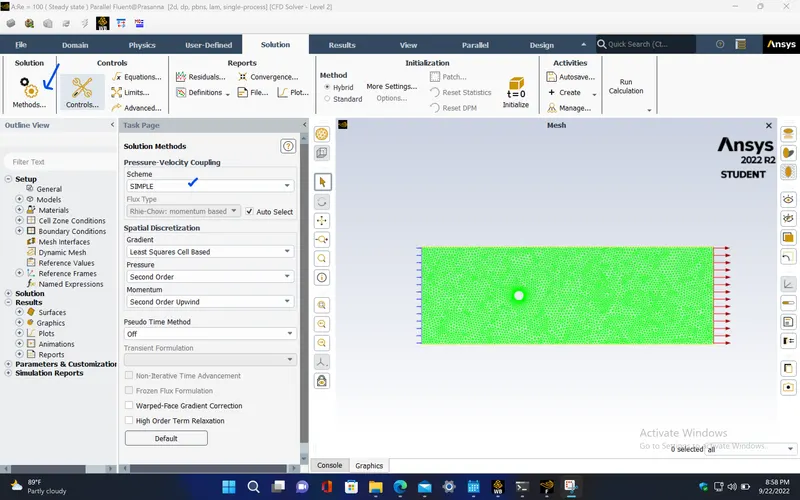
Pressure-Velocity Coupling
Type	SIMPLE

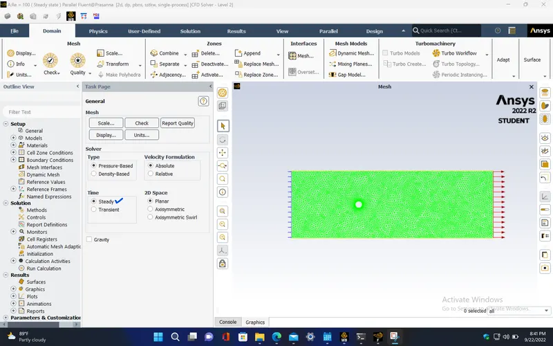
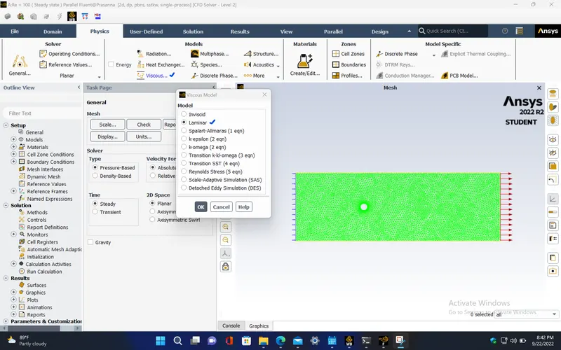
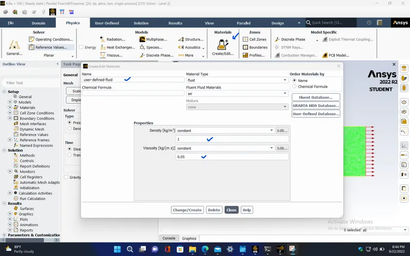
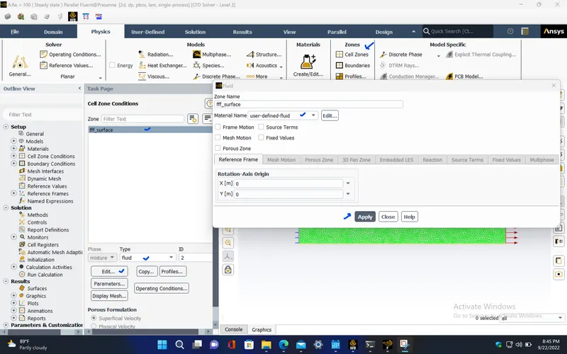
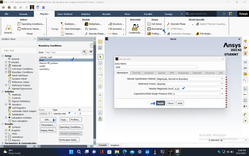
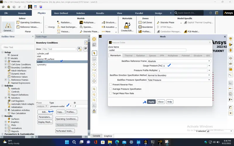
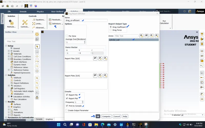
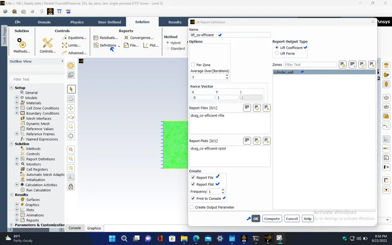
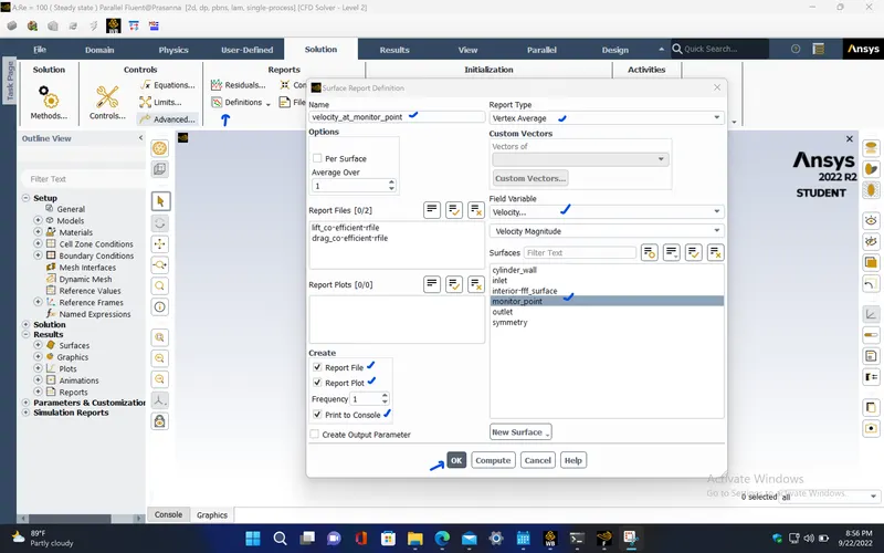
• Create report definitions for lift and drag co-efficient, and for the velocity at the monitor point.

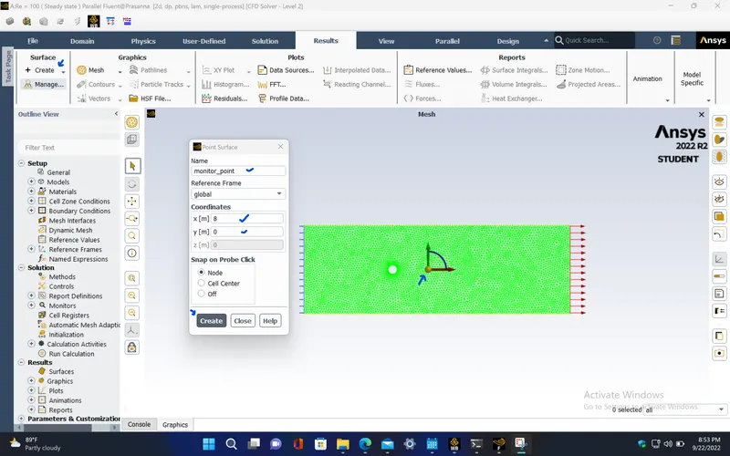
• Create monitor point at a distance of 4*D = 8 m behind the cylinder inorder to capture the velocity fluctuation due to vortex shedding.

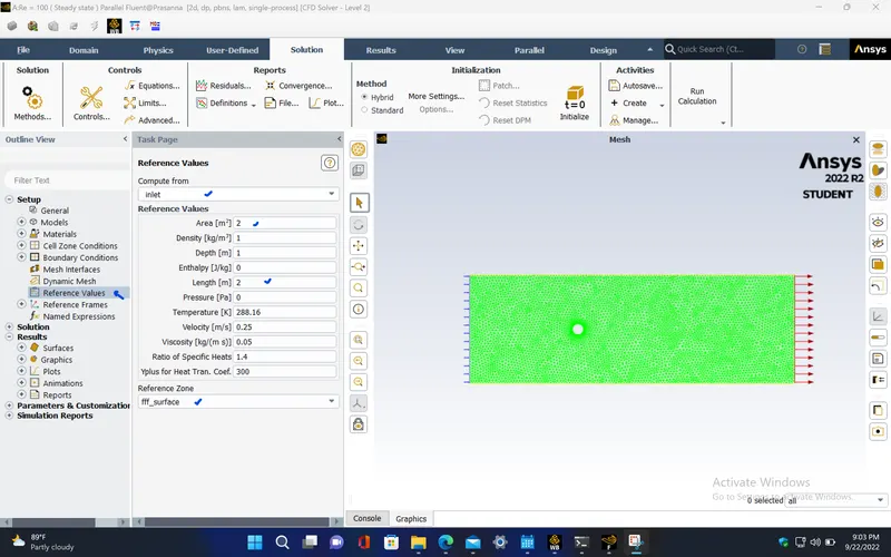
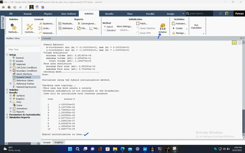
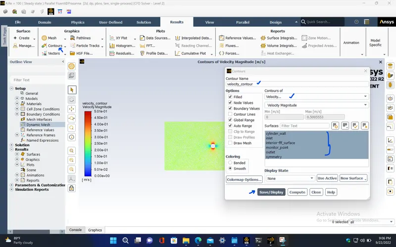
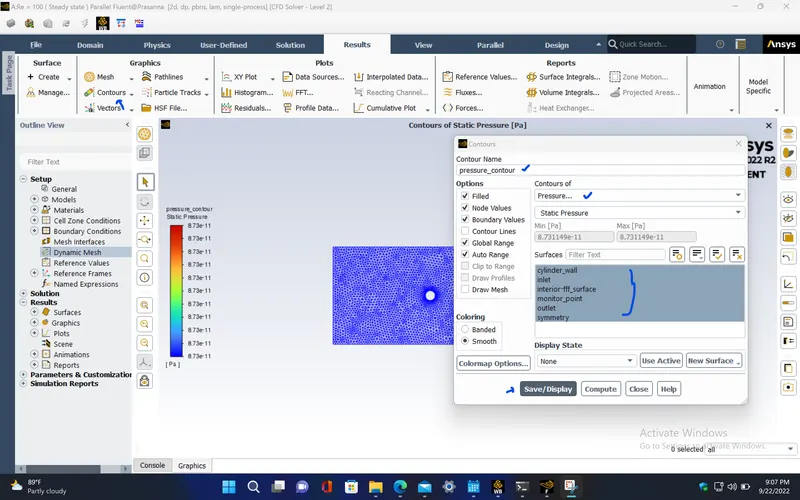
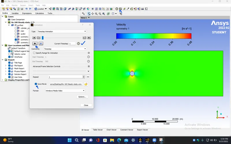
• To create animation, autosave the data for every iteration before starting the simulation.

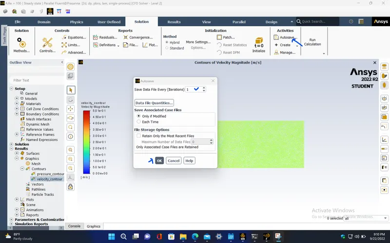
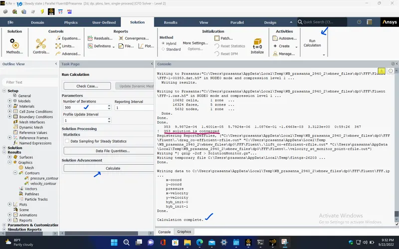
• Now, Run the simulation for 500 iterations.

RESIDUAL PLOT :

VELOCITY PLOT AT THE MONITOR POINT :

DRAG CO-EFFICIENT PLOT :

LIFT CO-EFFICIENT PLOT :

SOLUTION STATUS :

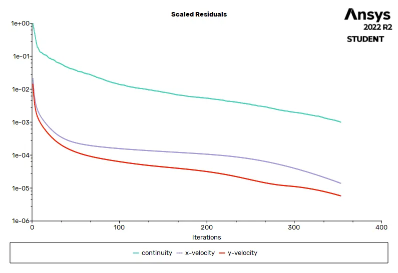
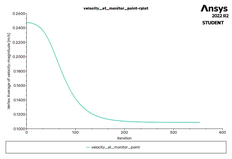
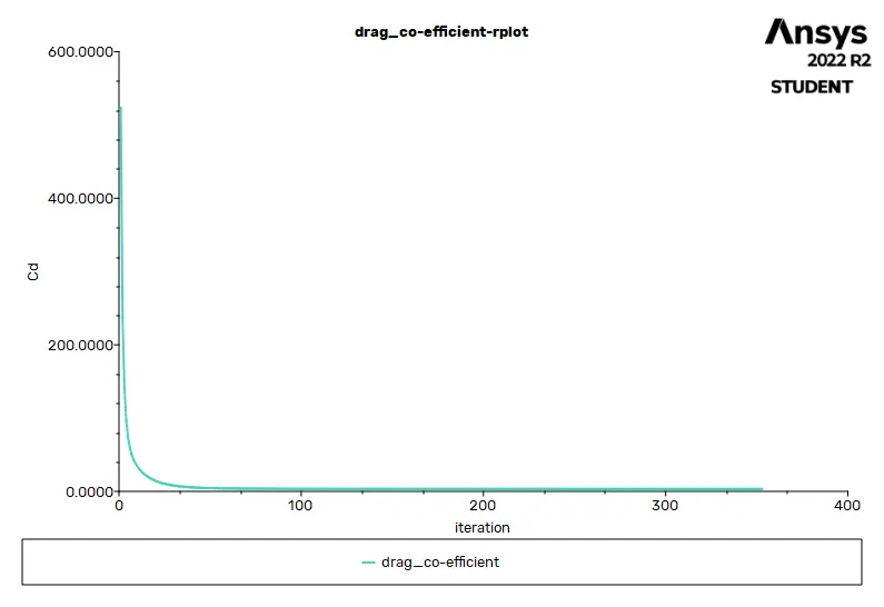
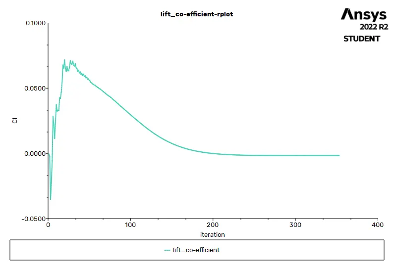
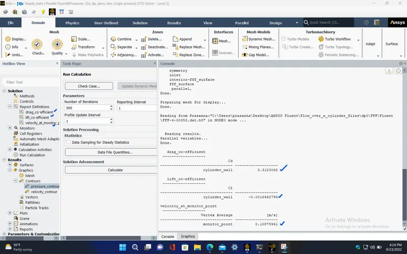
• From the above plots, we see that the solution got converged at 353th iteration since the rate at which residuals, velocity, drag co-efficient and lift co-efficient changes becomes constant over iteration.

Number of iteration - 353

	Value	Absolute Criteria	Convergence Status
continuity	0.000998717	0.001	Converged
x-velocity	1.400098e-05	0.001	Converged
y-velocity	5.792355e-06	0.001	Converged

REPORT DEFINITIONS :

velocity_at_monitor_point	0.1087596	m/s
lift_co-efficient	-0.00164628
drag_co-efficient	3.312306

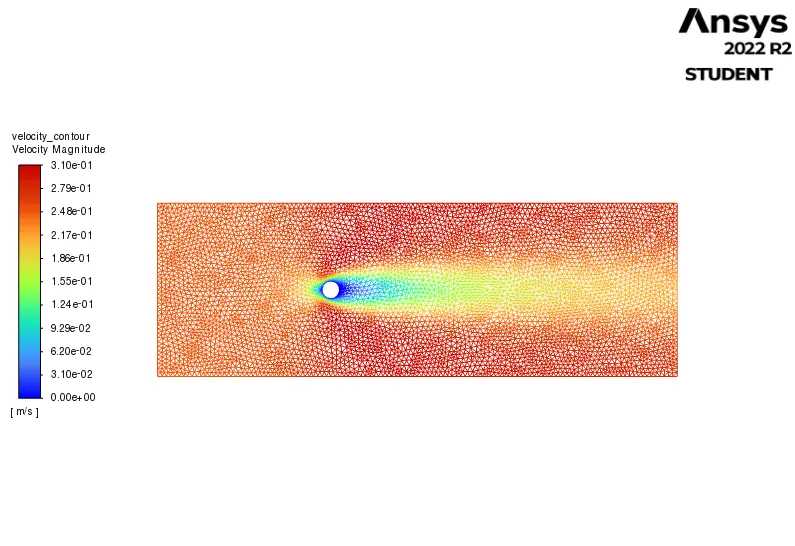
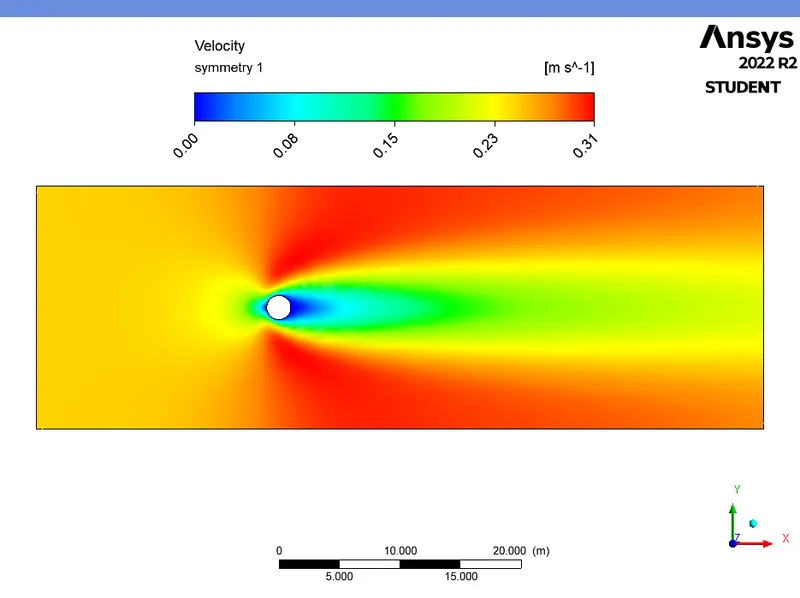
VELOCITY CONTOUR :

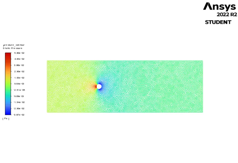
PRESSURE CONTOUR :

POST PROCESSING :

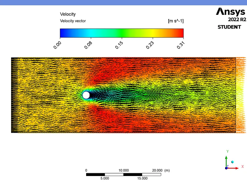
VELOCITY CONTOUR PLOT :

VELOCITY VECTOR PLOT :

• Now, Create the animation with the help of saved timesteps for the simulation

2. For Reynolds number = 100 (i.e,velocity = 2.5 m/s) Steady state :

• Repeat the same procedure as in previous case but now, change the inlet velocity of fluid to 2.5 m/s

BOUNDARY CONDITIONS :

inlet
Velocity Specification Method	Magnitude, Normal to Boundary
Reference Frame	Absolute
Velocity Magnitude [m/s]	2.5
Supersonic/Initial Gauge Pressure [Pa]	0
outlet
Backflow Reference Frame	Absolute
Gauge Pressure [Pa]	0
Backflow Direction Specification Method	Normal to Boundary

Symmetry
symmetry	symmetry
cylinder_wall
Wall Motion	Stationary Wall
Shear Boundary Condition	No Slip

REFERENCE VALUES :

Area	2 m^2
Density	1 kg/m^3
Depth	1 m
Enthalpy	0 J/kg
Length	2 m
Pressure	0 Pa
Temperature	288.16 K
Velocity	2.5 m/s
Viscosity	0.05 kg/(m s)
Ratio of Specific Heats	1.4
Yplus for Heat Tran. Coef.	300
Reference Zone	fff_surface

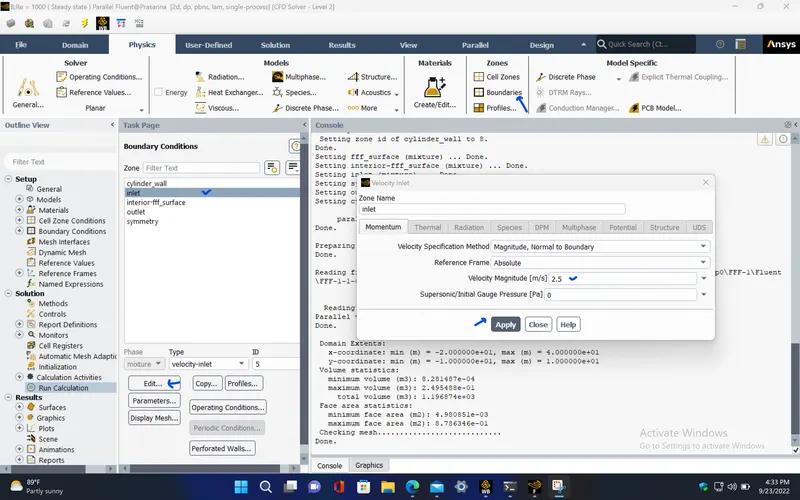
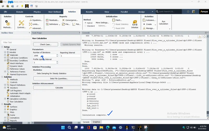
• Now, Run the simulation for 1000 iterations ( For capturing the vortex shedding behind cylinder and also to get the solution converged, I ran the simulation for 1000 iterations).

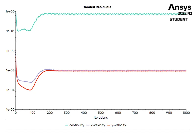
RESIDUAL PLOTS :

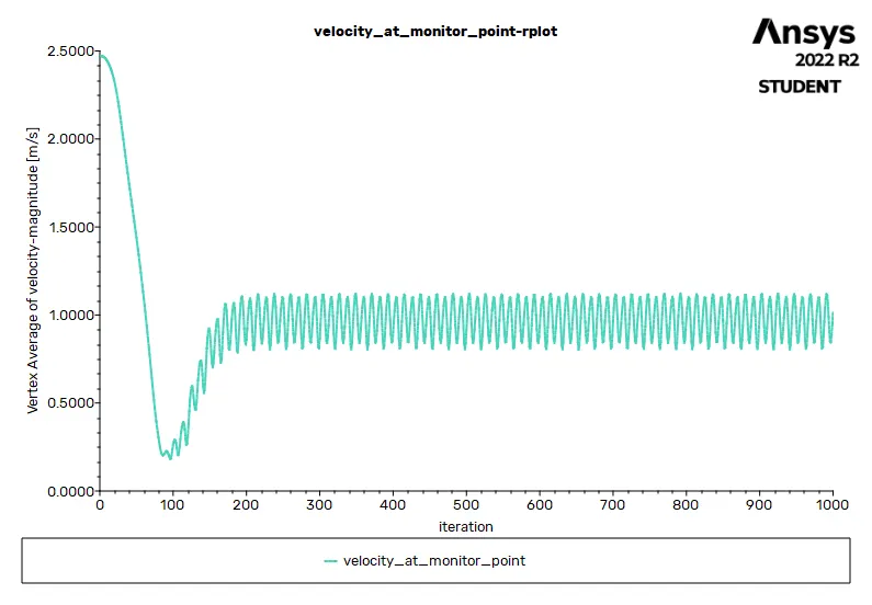
VELOCITY PLOT AT THE MONITOR POINT :

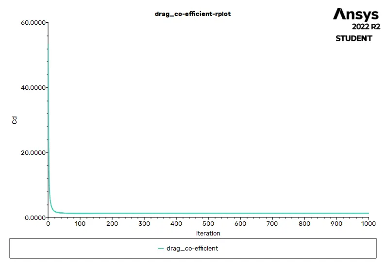
DRAG CO-EFFICIENT :

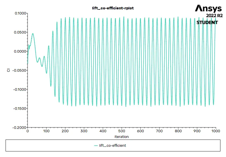
LIFT CO-EFFICIENT :

SOLUTION STATUS :

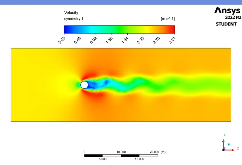
• From the above plots, we see that the solution got converged after 300 iterations since the rate at which velocity, drag co-efficient, and lift co-efficient changes becomes to a constant rate over iteration.

Number of iteration - 1000

	Value	Absolute Criteria	Convergence Status
continuity	0.7481465	0.001	Not Converged
x-velocity	0.0009941753	0.001	Converged
y-velocity	0.0009252606	0.001	Converged

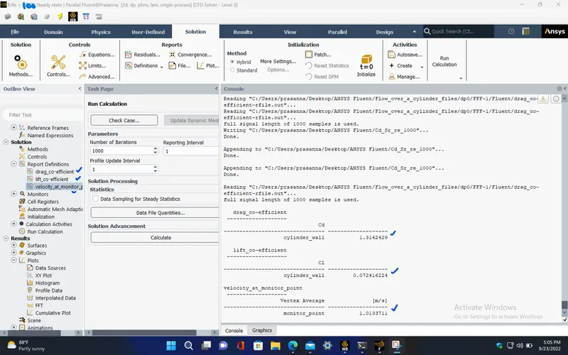
REPORT DEFINITIONS :

velocity_at_monitor_point	1.013371	m/s
lift_co-efficient	0.07241622
drag_co-efficient	1.314243

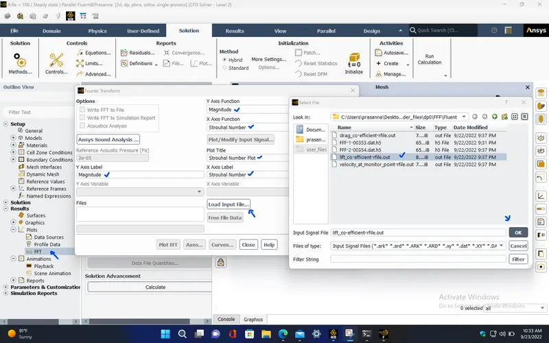
• To create the Strouhal number plot with its magnitude, use the lift co-efficient data file.

VELOCITY CONTOUR PLOT :

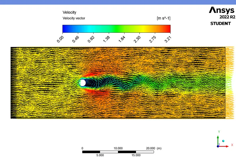
VELOCITY VECTOR PLOT :

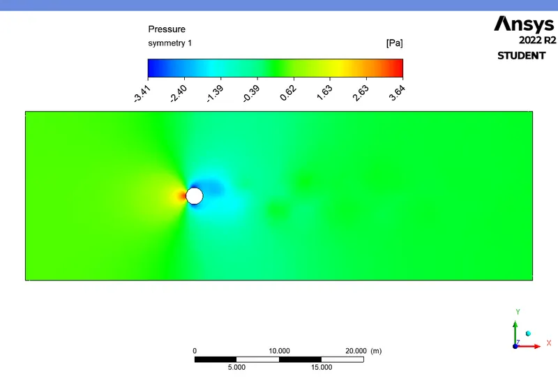
PRESSURE CONTOUR PLOT :

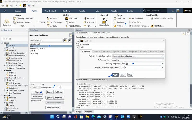
3. For Reynolds number = 1000 (i.e,velocity = 25 m/s) Steady state :

BOUNDARY CONDITIONS :

inlet
Velocity Specification Method	Magnitude, Normal to Boundary
Reference Frame	Absolute
Velocity Magnitude [m/s]	25
Supersonic/Initial Gauge Pressure [Pa]	0
outlet
Backflow Reference Frame	Absolute
Gauge Pressure [Pa]	0
Backflow Direction Specification Method	Normal to Boundary

Symmetry
symmetry	symmetry
Wall
cylinder_wall
Wall Motion	Stationary Wall
Shear Boundary Condition	No Slip

REFERENCE VALUES :

Area	2 m^2
Density	1 kg/m^3
Depth	1 m
Enthalpy	0 J/kg
Length	2 m
Pressure	0 Pa
Temperature	288.16 K
Velocity	25 m/s
Viscosity	0.05 kg/(m s)
Ratio of Specific Heats	1.4
Yplus for Heat Tran. Coef.	300
Reference Zone	fff_surface

• Now, Run the simulation for 1000 iterations ( For capturing the vortex shedding behind cylinder and also to get the solution converged, I ran the simulation for 1000 iterations).

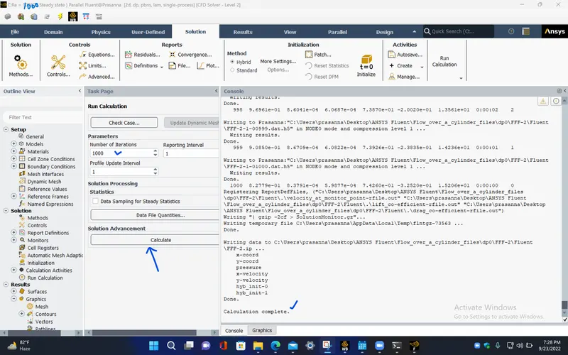
RESIDUAL PLOTS :

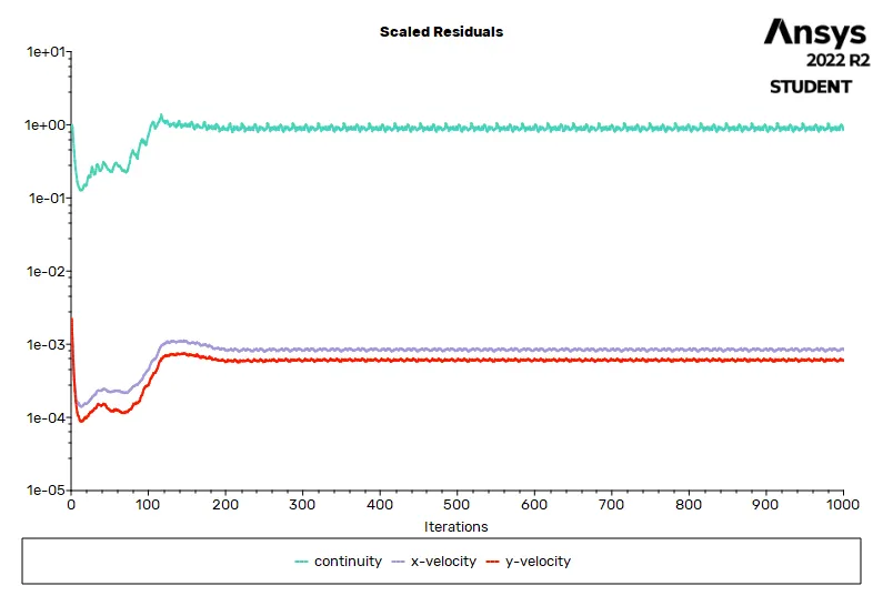
VELOCITY PLOT AT THE MONITOR POINT :

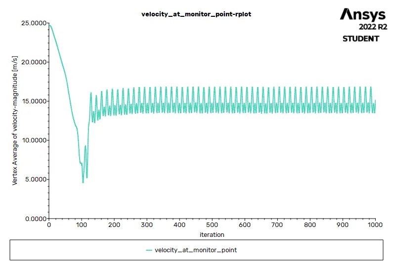
DRAG CO-EFFICIENT :

LIFT CO-EFFICIENT :

SOLUTION STATUS :

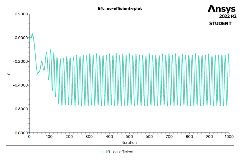
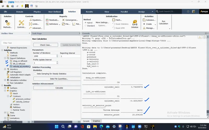
• From the above plots, we see that the solution got converged after 300 iterations since the rate at which velocity, drag co-efficient, and lift co-efficient changes becomes to a constant rate over iteration.

Number of iteration - 1000

	Value	Absolute Criteria	Convergence Status
continuity	0.8277872	0.001	Not Converged
x-velocity	0.0008379091	0.001	Converged
y-velocity	0.0005987713	0.001	Converged

REPORT DEFINITIONS :

drag_co-efficient	0.7425958
lift_co-efficient	-0.3251965
velocity_at_monitor_point	15.20617	m/s

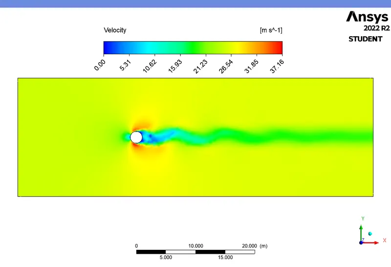
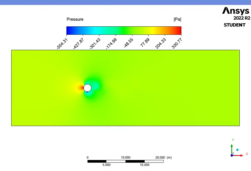
VELOCITY CONTOUR PLOT :

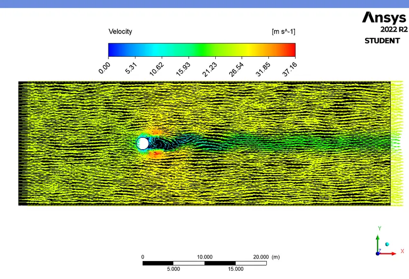
VELOCITY VECTOR PLOT :

PRESSURE CONTOUR PLOT :

4. For Reynolds number = 10000 (i.e,velocity = 250 m/s) Steady state :

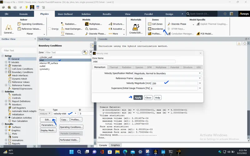
BOUNDARY CONDITIONS :

inlet
Velocity Specification Method	Magnitude, Normal to Boundary
Reference Frame	Absolute
Velocity Magnitude [m/s]	250
Supersonic/Initial Gauge Pressure [Pa]	0
outlet
Backflow Reference Frame	Absolute
Gauge Pressure [Pa]	0
Backflow Direction Specification Method	Normal to Boundary

Symmetry
symmetry	symmetry
Wall
cylinder_wall
Wall Motion	Stationary Wall
Shear Boundary Condition	No Slip

REFERENCE VALUES :

Area	2 m^2
Density	1 kg/m^3
Depth	1 m
Enthalpy	0 J/kg
Length	2 m
Pressure	0 Pa
Temperature	288.16 K
Velocity	250 m/s
Viscosity	0.05 kg/(m s)
Ratio of Specific Heats	1.4
Yplus for Heat Tran. Coef.	300
Reference Zone	fff_surface

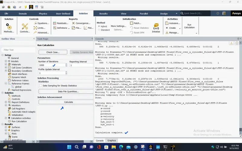
• Now, Run the simulation for 1000 iterations ( For capturing the vortex shedding behind cylinder and also to get the solution converged, I ran the simulation for 1000 iterations).

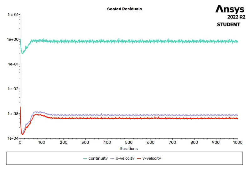
RESIDUAL PLOTS :

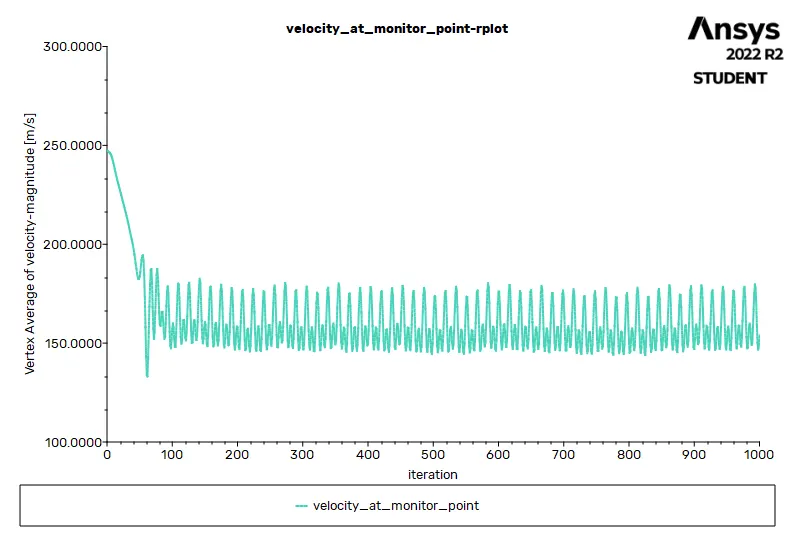
VELOCITY PLOT AT THE MONITOR POINT :

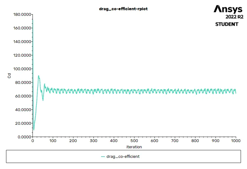
DRAG CO-EFFICIENT PLOT :

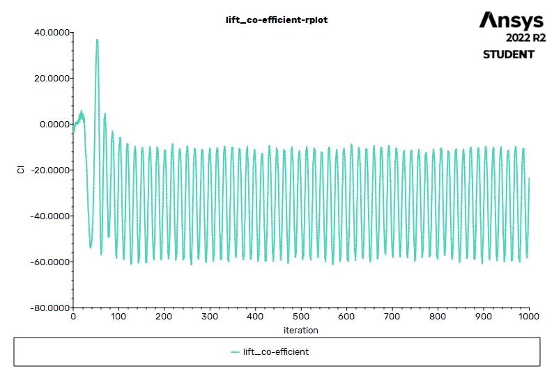
LIFT CO-EFFICIENT PLOT :

SOLUTION STATUS :

• From the above plots, we see that the solution got converged after 300 iterations since the rate at which velocity, drag co-efficient, and lift co-efficient changes becomes to a constant rate over iteration.

Number of iteration - 1000

	Value	Absolute Criteria	Convergence Status
continuity	0.7773383	0.001	Not Converged
x-velocity	0.0008316889	0.001	Converged
y-velocity	0.0006289721	0.001	Converged

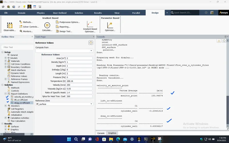
REPORT DEFINITIONS :

velocity_at_monitor_point	153.9457	m/s
lift_co-efficient	-0.2346141
drag_co-efficient	0.6383622

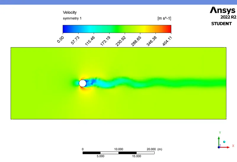
VELOCITY CONTOUR PLOT :

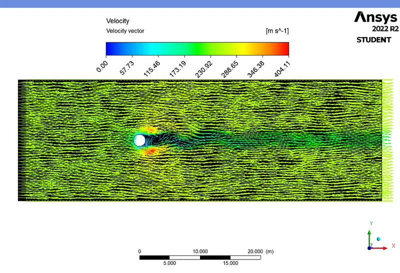
VELOCITY VECTOR PLOT :

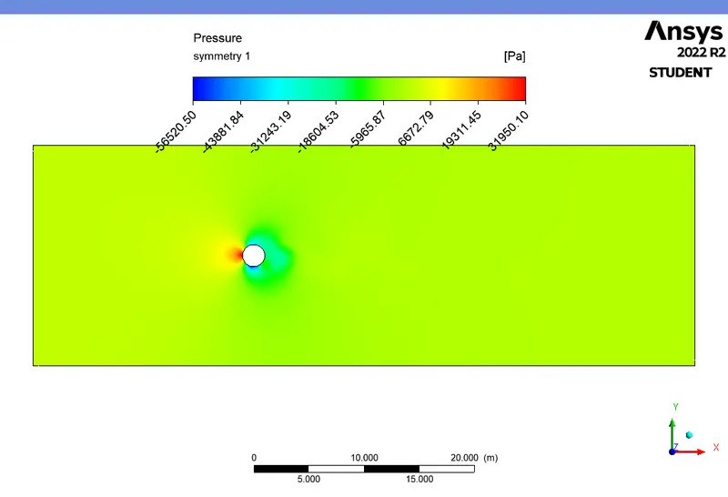
PRESSURE CONTOUR PLOT :

5. For Reynolds number = 100000 (i.e,velocity = 2500 m/s) Steady state :

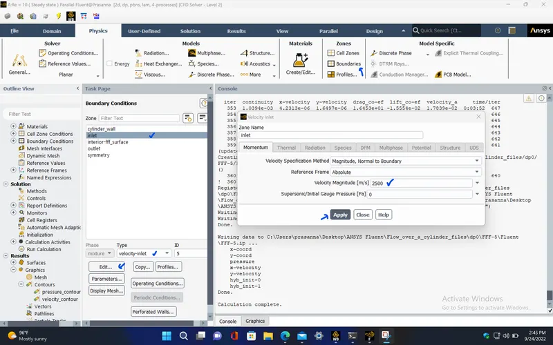
BOUNDARY CONDITIONS :

inlet
Velocity Specification Method	Magnitude, Normal to Boundary
Reference Frame	Absolute
Velocity Magnitude [m/s]	2500
Supersonic/Initial Gauge Pressure [Pa]	0
outlet
Backflow Reference Frame	Absolute
Gauge Pressure [Pa]	0
Backflow Direction Specification Method	Normal to Boundary

Symmetry
symmetry	symmetry
cylinder_wall
Wall Motion	Stationary Wall
Shear Boundary Condition	No Slip

REFERENCE VALUES :

Area	2 m^2
Density	1 kg/m^3
Depth	1 m
Enthalpy	0 J/kg
Length	2 m
Pressure	0 Pa
Temperature	288.16 K
Velocity	2500 m/s
Viscosity	0.05 kg/(m s)
Ratio of Specific Heats	1.4
Yplus for Heat Tran. Coef.	300
Reference Zone	fff_surface

• Now, Run the simulation for 1000 iterations ( For capturing the vortex shedding behind cylinder and also to get the solution converged, I ran the simulation for 1000 iterations).

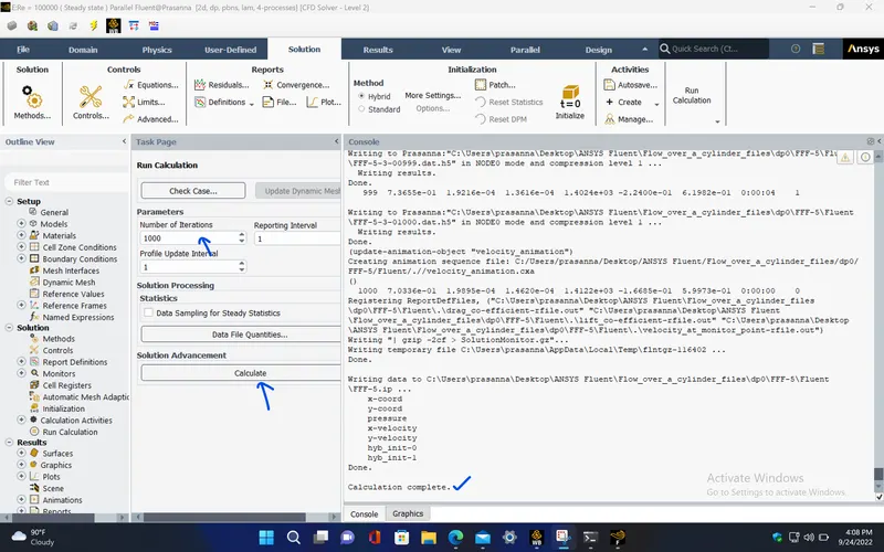
RESIDUAL PLOTS :

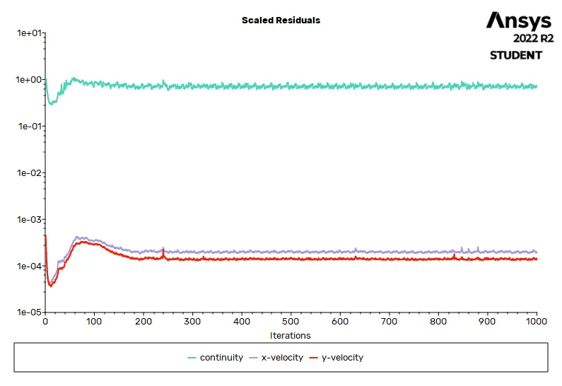
VELOCITY PLOT AT THE MONITOR POINT :

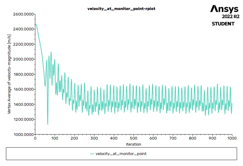
DRAG CO-EFFICIENT PLOT :

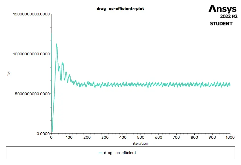
LIFT CO-EFFICIENT PLOT :

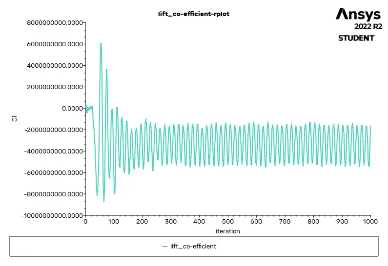
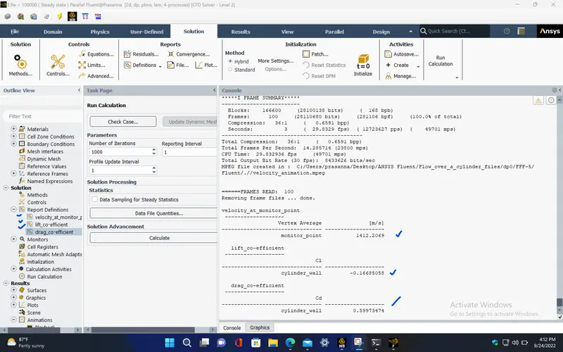
SOLUTION STATUS :

• From the above plots, we see that the solution got converged after 400 iterations since the rate at which velocity, drag co-efficient, and lift co-efficient changes becomes to a constant rate over iteration.

Number of iterations - 1000

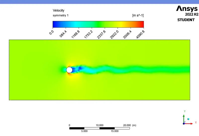
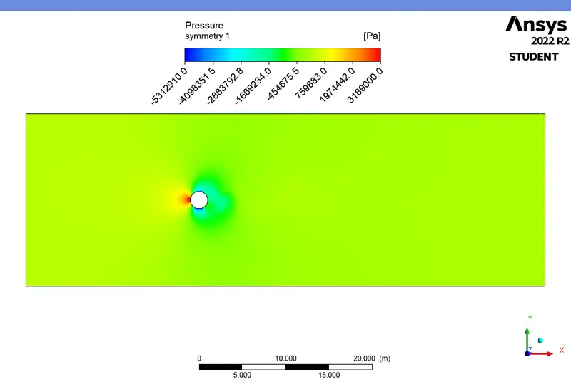
VELOCITY CONTOUR PLOT :

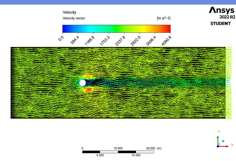
VELOCITY VECTOR PLOT :

PRESSURE CONTOUR PLOT :

6. For Reynolds number = 100 (i.e,velocity = 2.5 m/s) Transient state :

Model	Settings
Time	Unsteady, 1st-Order Implicit
Viscous	Laminar

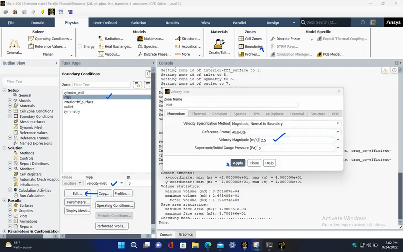
BOUNDARY CONDITIONS :

inlet
Velocity Specification Method	Magnitude, Normal to Boundary
Reference Frame	Absolute
Velocity Magnitude [m/s]	2.5
Supersonic/Initial Gauge Pressure [Pa]	0
outlet
Backflow Reference Frame	Absolute
Gauge Pressure [Pa]	0
Backflow Direction Specification Method	Normal to Boundary

Symmetry
symmetry	symmetry
Wall
cylinder_wall
Wall Motion	Stationary Wall
Shear Boundary Condition	No Slip

REFERENCE VALUES :

Area	2 m^2
Density	1 kg/m^3
Depth	1 m
Enthalpy	0 J/kg
Length	2 m
Pressure	0 Pa
Temperature	288.16 K
Velocity	2.5 m/s
Viscosity	0.05 kg/(m s)
Ratio of Specific Heats	1.4
Yplus for Heat Tran. Coef.	300
Reference Zone	fff_surface

SOLVER :

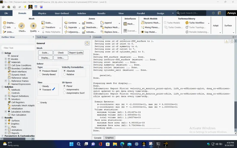
Unsteady Calculation Parameters
Number of Time Steps	1000
Time Step Size [s]	0.1
Max Iterations/Time Step	20
Pressure-Velocity Coupling
Type	SIMPLE

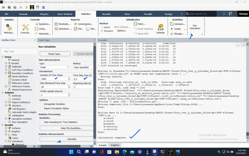
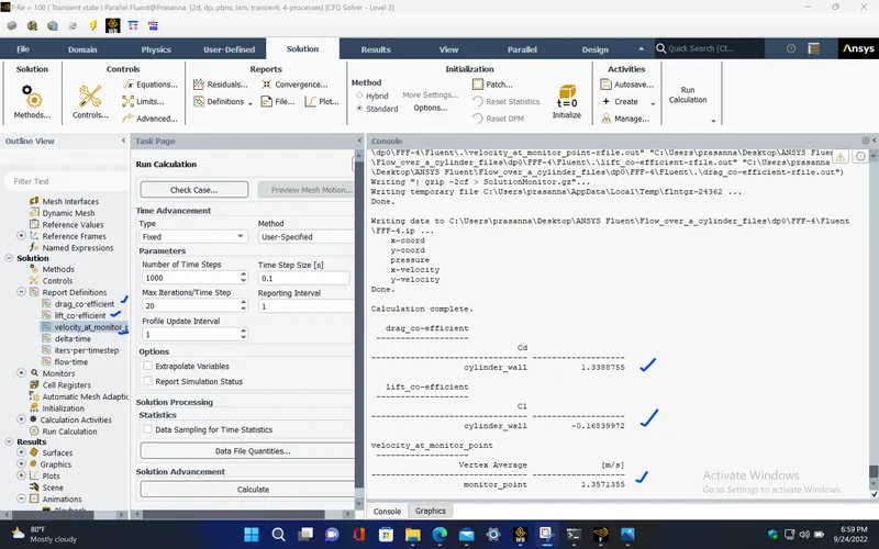
• Now, Run the simulation for 1000 number of time steps with 0.1 as time step size which gives 100 seconds ( This is done for capturing the vortex shedding behind cylinder and also to get the solution converged).

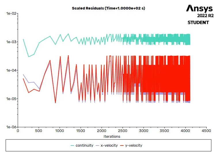
RESIDUAL PLOTS :

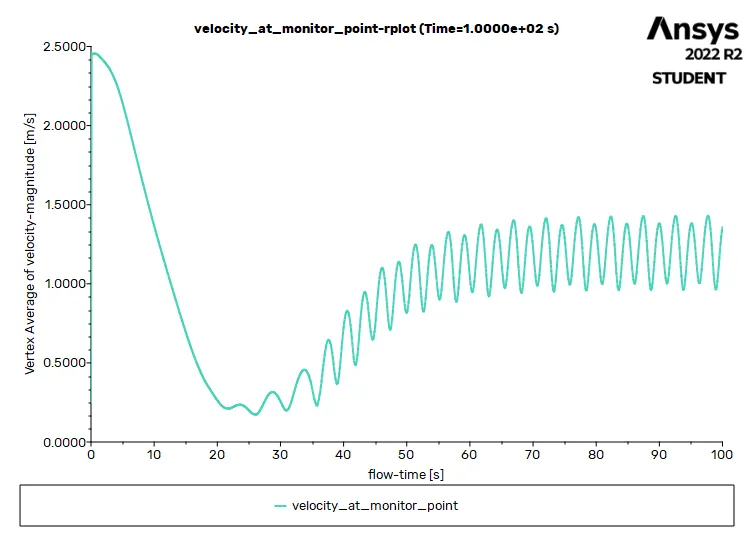
VELOCITY PLOT AT THE MONITOR POINT :

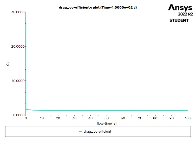
DRAG CO-EFFICIENT PLOT :

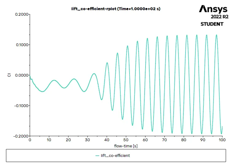
LIFT CO-EFFICIENT PLOT :

SOLUTION STATUS :

• From the above plots, we see that the solution got converged after 60 seconds since the rate at which residuals, velocity, drag co-efficient, and lift co-efficient changes becomes to a constant rate over time.

	Value	Absolute Criteria	Convergence Status
continuity	0.0007884178	0.001	Converged
x-velocity	7.269933e-06	0.001	Converged
y-velocity	8.632251e-06	0.001	Converged

REPORT DEFINITIONS :

drag_co-efficient	1.338876
lift_co-efficient	-0.1683997
velocity_at_monitor_point	1.357136	m/s
delta-time	0.1	s
iters-per-timestep	6
flow-time	100	s

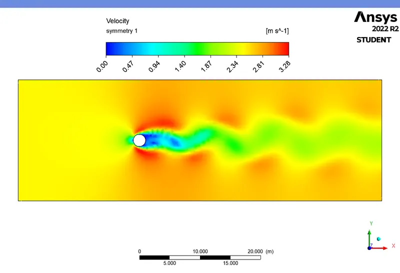
VELOCITY CONTOUR PLOT :

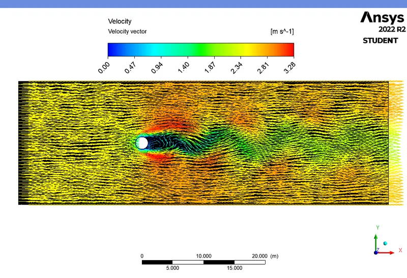
VELOCITY VECTOR PLOT :

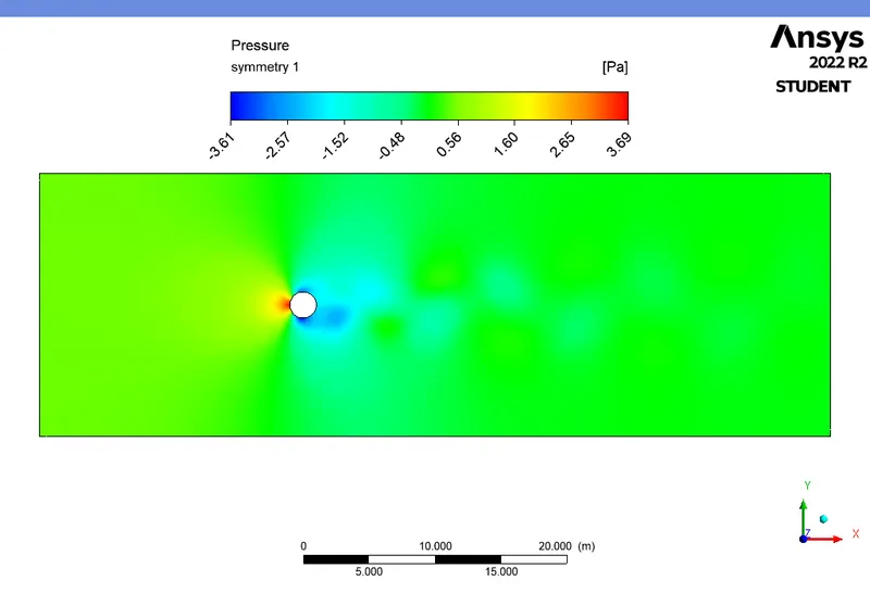
PRESSURE CONTOUR PLOT :

RESULTS :

Google drive link :

https://drive.google.com/file/d/1b0okBgzoK1GsWTGUi89WHhrqc0y_AQVj/view?usp=sharing

1. STROUHAL NUMBER PLOT : (Steady state with Reynolds number - 100)

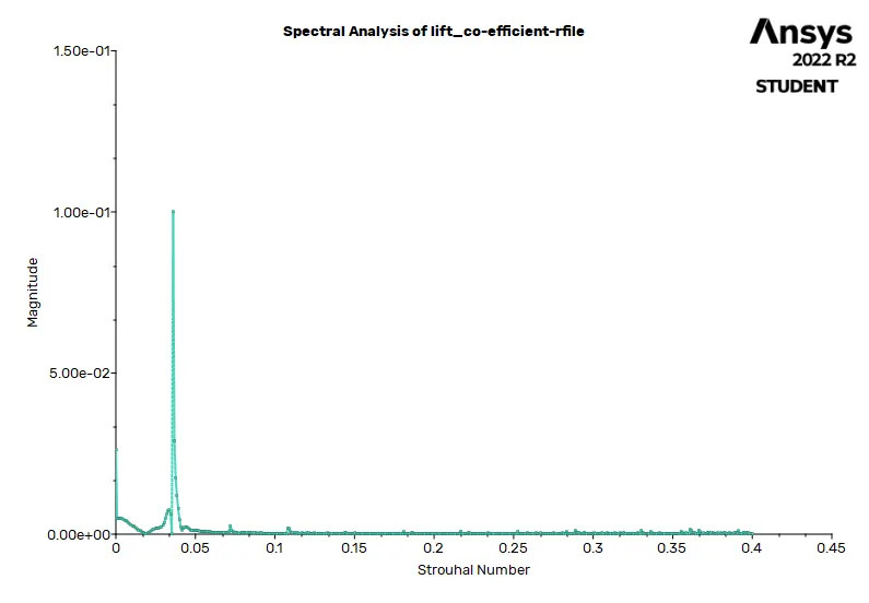
• Sr = 0.14

2. STROUHAL NUMBER PLOT : (Transient state with Reynolds number - 100)

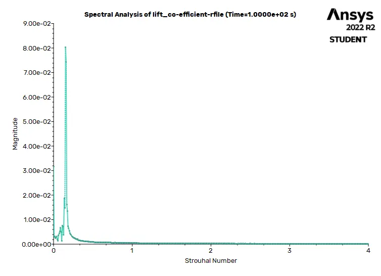
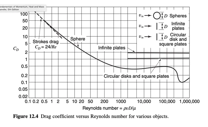
Effect of Reynolds number on the coefficient of drag :

This screenshots is taken from the standard literature to validate the simulated result,

FINAL SOLUTION :

Reynolds number	Drag co-efficient
10	3.312306
100	1.314243
1000	0.7425958
10000	0.6383622
100000	0.59973474

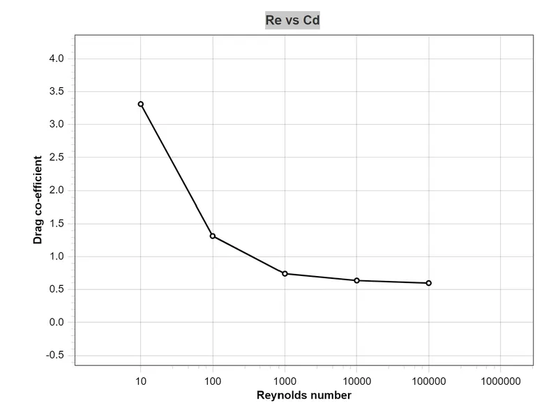
CONCLUSION :

From the above plot, we can state that for a flow over a cylinder as Reynolds number increases, the drag co-efficient decreases. Also, we know that co-efficient of drag is inversely proportional to the velocity square of thre fluid flow. Thus, we get the required result.

REFERENCE :

1. https://commons.wikimedia.org/wiki/File:Drag_Coefficient_(Cd)_vs_Reynolds_number_(Re)_in_various_objects.png

2. https://www.sciencedirect.com/science/article/pii/S0307904X08000243

3. https://www.researchgate.net/figure/The-drag-coefficient-C-D-for-a-circular-cylinder-subjected-to-cross-flow-as-a_fig3_241449048