Week 5 - Rayleigh Taylor Instability
AIM :
To perform the Rayleigh Taylor instability simulation for two dimensional multiphase flow of two immiscible fluids (water and air in one case, water and user defined fluid for the other).
OBJECTIVES :
- To create two dimensional surfaces for the two fluid components in spaceclaim.
- To generate mesh with different mesh element size for different cases and perform the mesh independency study for those cases.
- To setup the simulation for capturing the Rayleigh Taylor instability between the two immiscible fluids which flows due to gravity.
- To create animation for visualising the Rayleigh instability on those fluids and to calculate the Atwood number for water and air, also water and user defined fluid.
INTRODUCTION :
In this project, we are going to perform the two dimensional simulation for two immiscible fluids that have different densities. Initially, the fluid with high density is placed at the top region while the fluid having lesser density at the bottom. Due to gravity, the heavy dense fluid flows downwards making the less dense fluid to go up. This causes the Rayleigh Taylor instability between the interface of those two fluids. This instability is captured from this simulation which set to run at transient state with maximum of 10 flow seconds in some cases which is more than enough for the two fluids to reach the steady state.
Reason for using Transient state over steady state for this simulation,
Here, we use transient (Unsteady) state for this simulation and not the steady state. This is because, the steady state simulation gives the final state that is reached by those fluids. So, simulating with steady state will try to solve for the final state solution of the fluids for each iteration where, in transient case, the flow is captured for each time steps which gives the exact solution at that time of the simulation.
CFD MODELS BASED ON RAYLEIGH-TAYLOR WAVES :
Rayleigh-Taylor instability :
It is an instability of an interface between two fluids of different densities which occurs when the lighter fluid is pushing the heavier fluid. For example, If the water is suspended above oil which has less density than water, due to gravity, the heavier dense water flows downwards which makes the oil to go upwards. This behaviour is Rayleigh instability.
Richtmeyer-Meshkow instability :
This instability occurs when a shock wave interacts with an interface separating two different fluids or in other words when two fluids of different densities are impulsively accelerated.The development of instability begins with small amplitude which initially grow linear with time. This is followed by a nonlinear regime with bubbles appearing in the case of a light fluid penetrating a heavy fluid, and with spikes appearing in the case of a heavy fluid penetrating a light fluid. A chaotic regime eventually is reached and the two fluids mixThis instability can be considered the impulsive acceleration limit of the Rayleigh Taylor Instability.
Plateau-Rayleigh instability :
This instability explains why and how a falling stream of fluid breaks up into smaller packets with the same volume but different or small surface area.The driving force of this instability is that the liquids by virtue of their surface tensions ,tends to minimize their surface area .
Kelvin-Helmholtz instability :
This instability can occur when there is velocity shear in a single continuous fluid, or where there is a velocity difference across the interface between two fluids. For example, wind blowing over the water, cloud formation, etc.
ATWOOD NUMBER :
It is a dimensionless number which is defined as the ratio of the difference between the heavier fluid density and the lighter fluid density to their sum. It used in the study of hydrodynamic instabilities in density stratified flows. It is an important parameter in the study of Rayleigh-Taylor instability and Richtmyer-Meshkov instability.
- `"Atwood number (A)" = (rho_1 - rho_2) / (rho_1 + rho_2)`
Where,
- `rho_1 = "Density of the heavier fluid"`
- `rho_2 = "Density of the lighter fluid"`
CALCULATION OF ATWOOD NUMBER :
1. For water and air,
Here, water is the heavier dense fluid compared to air, so, we take
Density of water,
`rho_1 = 998.2" kg/m^3"`
Density of air,
`rho_2 = 1.225" kg/m^3"`
We know that,
`"Atwood number (A)" = (rho_1 - rho_2) / (rho_1 + rho_2)`
`A = (998.2 - 1.225) / (998.2 + 1.225)`
`A = 0.9975`
2. For water and user defined fluid,
Density of user defined fluid,
`rho_2 = 400" kg/m^3"`
Density of water,
`rho_1 = 998.2" kg/m^3"`
Therefore,
`A = (998.2 - 400) / (998.2 + 400)`
`A = 0.4278`
CASE SETUP :
For this simulation, we are performing the mesh independency study for the case of water and air with three different mesh element lengths. Then, we choose a refined mesh element size for performing Rayleigh instability simulation on water and the user defined fluid which has the density of 400 kg/m^3 and viscosity of 0.001 kg/m-s.
| FLUIDS | MESH ELEMENT SIZE (in 'mm') | |
| CASE - 1 | Water and Air | 0.5 |
| CASE - 2 | Water and Air | 0.3 |
| CASE - 3 | Water and Air | 0.1 (Refined) |
| CASE - 4 | Water and User defined fluid | 0.1 (Refined) |
PROCEDURE :
CASE - 1 (Water and Air, Mesh element size as 0.5 mm) :
PRE-PROCESSING :
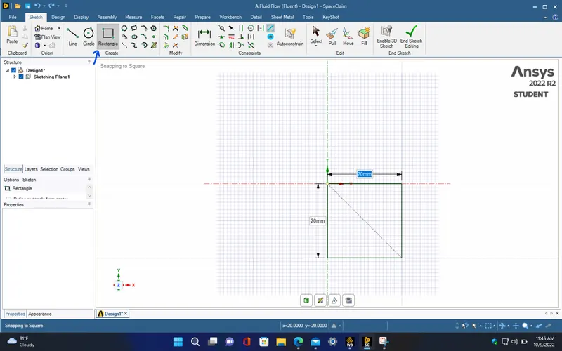
- Open spaceclaim from Ansys fluent flow in workbench. Then, select the XY plane as the sketch plane and create a square of 20mmX20mm from the origin towards the positive x-axis and negative y-axis direction.
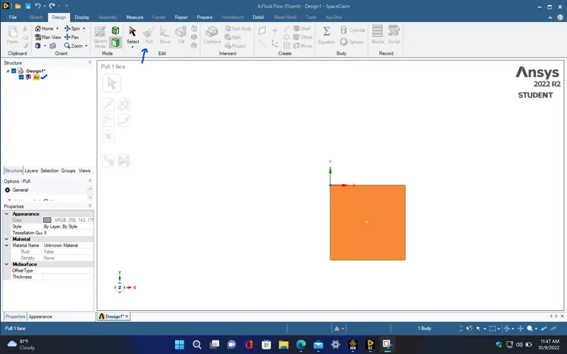
- Use the pull tool to convert the geometry into a surface and name it as air.
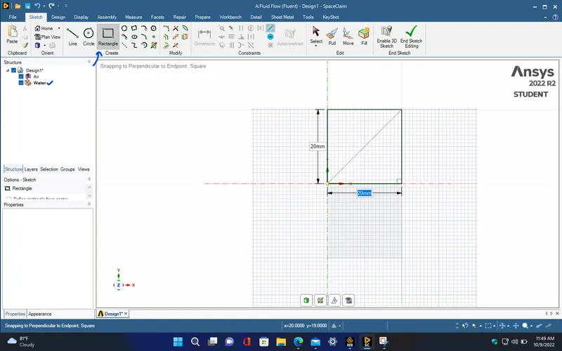
- Now, create another square above the previous surface of same dimension.
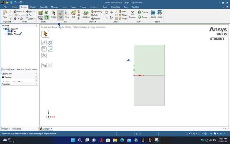
- Convert this geometry into a surface using the pull tool same as before.
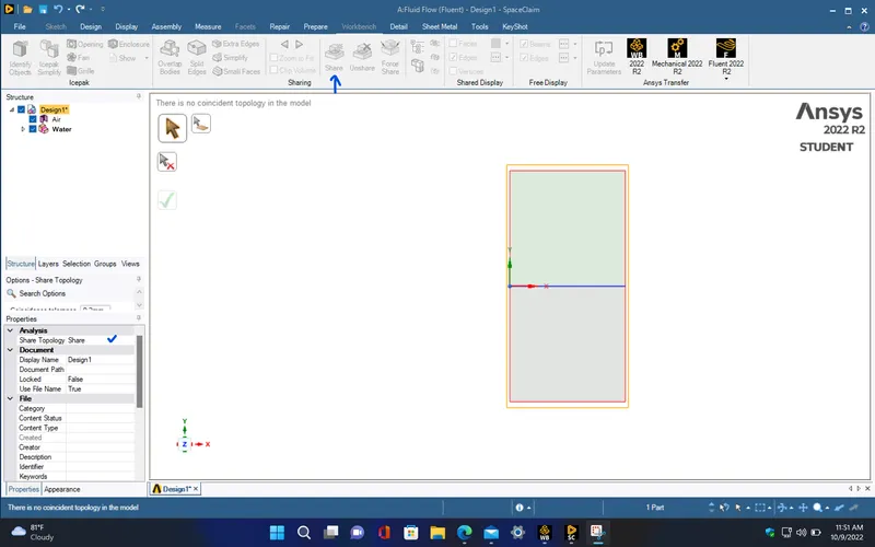
- Use share topology to share the common edge between the two surfaces and close spaceclaim.
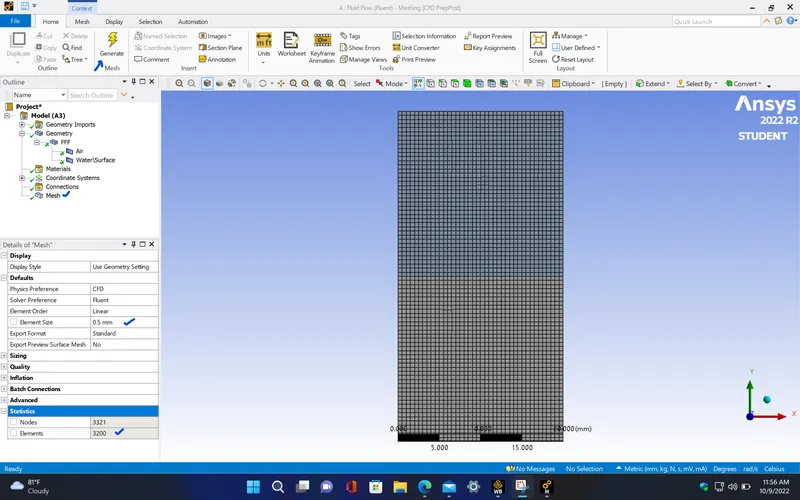
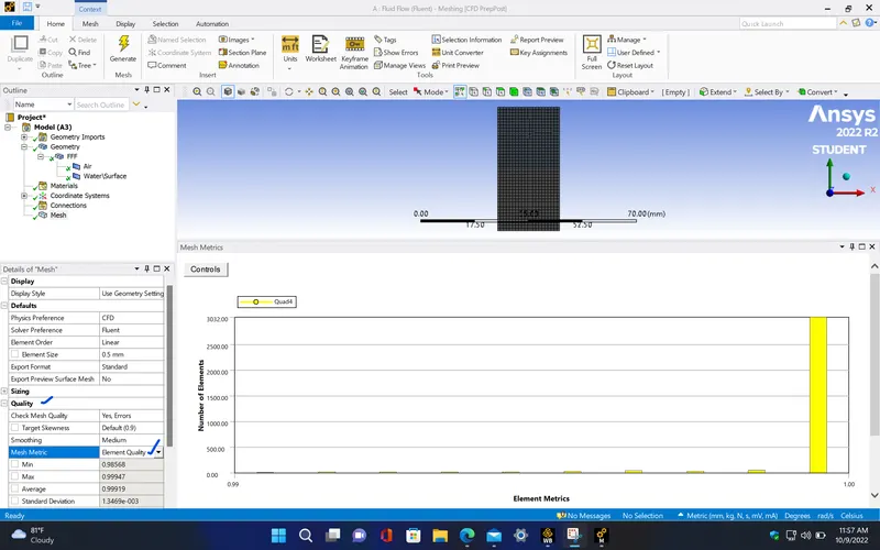
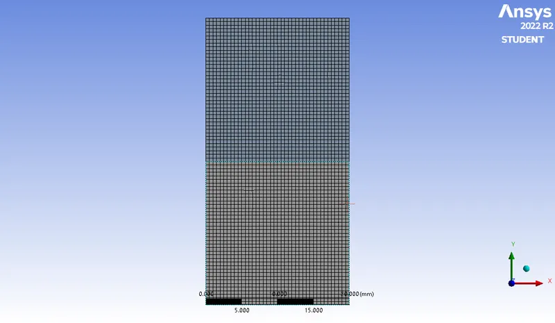
- Now, open mesh window from Ansys fluent. Give the element size as 5 mm and generate the mesh.
|
Cells |
Faces |
Nodes |
|
3200 |
6520 |
3321 |
SETUP AND SOLVING :
- Setup the problem by selecting the multiphase solver and volume of fluid method for this simulation. The parameters which are chosen are as follows,
|
Model |
Settings |
|
Space |
2D |
|
Time |
Unsteady, 1st-Order Implicit |
|
Model |
Settings |
|
Viscous |
Laminar |
|
Multiphase |
Volume of Fluid |
Material properties :
|
Fluid |
water-liquid |
|
Density |
998.2 kg/m^3 |
|
Cp (Specific Heat) |
4182 J/(kg K) |
|
Thermal Conductivity |
0.6 W/(m K) |
|
Viscosity |
0.001003 kg/(m s) |
|
Molecular Weight |
18.0152 kg/kmol |
|
Fluid |
air |
|
Density |
1.225 kg/m^3 |
|
Cp (Specific Heat) |
1006.43 J/(kg K) |
|
Thermal Conductivity |
0.0242 W/(m K) |
|
Viscosity |
1.7894e-05 kg/(m s) |
|
Molecular Weight |
28.966 kg/kmol |
Solver :
|
Pressure-Velocity Coupling |
SIMPLE |
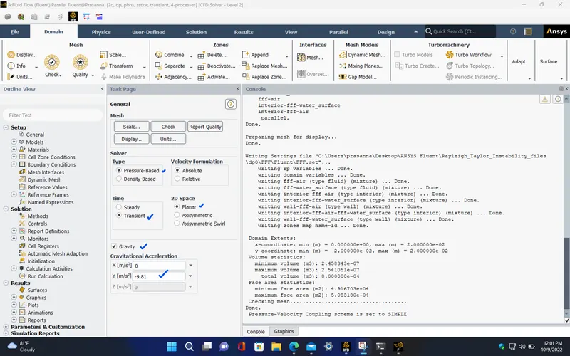
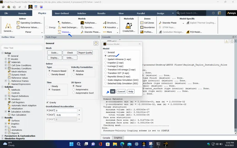
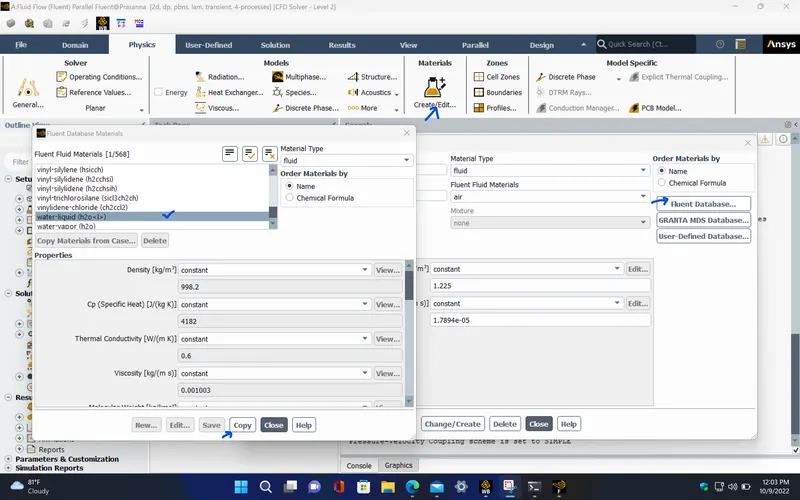
- To add water and its properties into the fluent materials, open fluent database. Select water-liquid from the list of fluent fluid materials and click copy. This will add the water to the current fluid materials.
- Select volume of fluid method from multiphase model, which is a surface tracking method used to find out the position of interface between any two or more immiscible fluids. The volume fraction of each fluid in each cell through out the domain is tracked. Also, Here we choose the implicit formulation scheme so that the time step size won't be a constraint in order to satisfy the courant number.
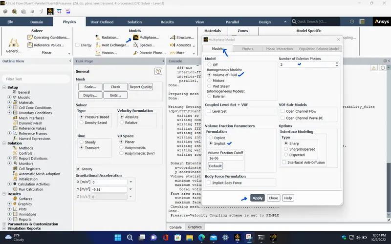
- Under phases tab, Choose air as the primary phase and water as the secondary phase.
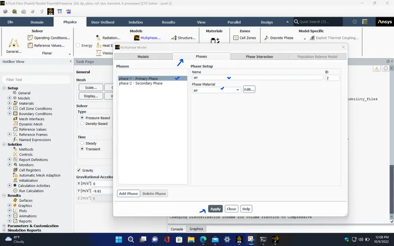
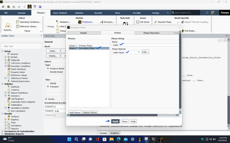
- Initialize the solution.
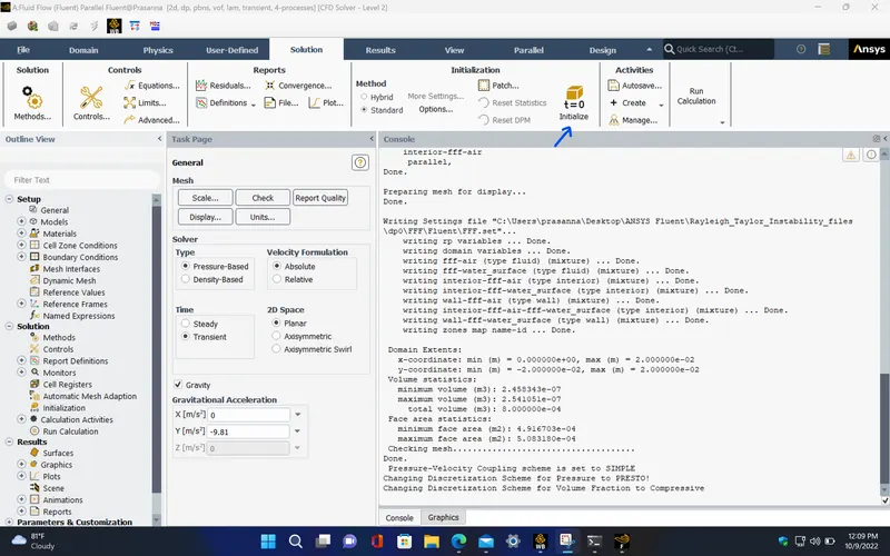
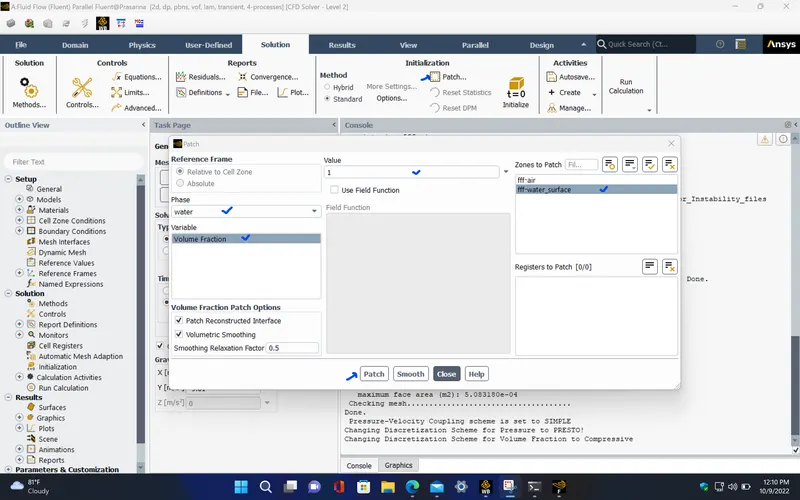
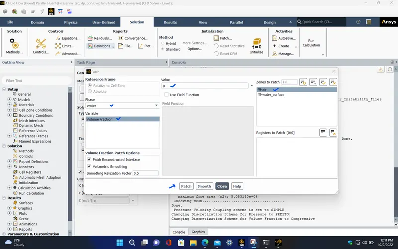
- After initialization, patch the fluids. Give the volume fraction value as 1 for the water phase at the water surface region(top region) and patch it. Then, give the volume fraction value as 0 for the water phase at the air surface region(bottom region) and patch. This ensures that, initially, the water is 100% at the water surface (top) and 0% at the air surface (bottom).
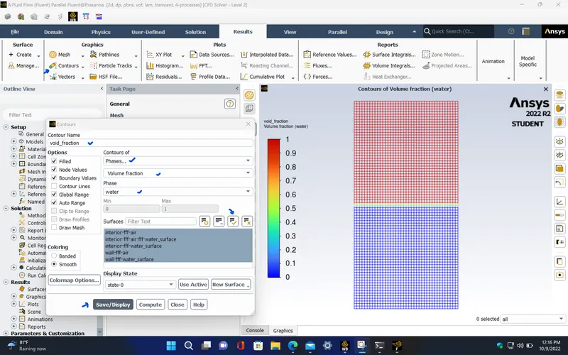
- To check if the fluids are patched properly, create contour for the volume fraction under phases, select the water phase and select the all the surfaces. Now, click save and display option.
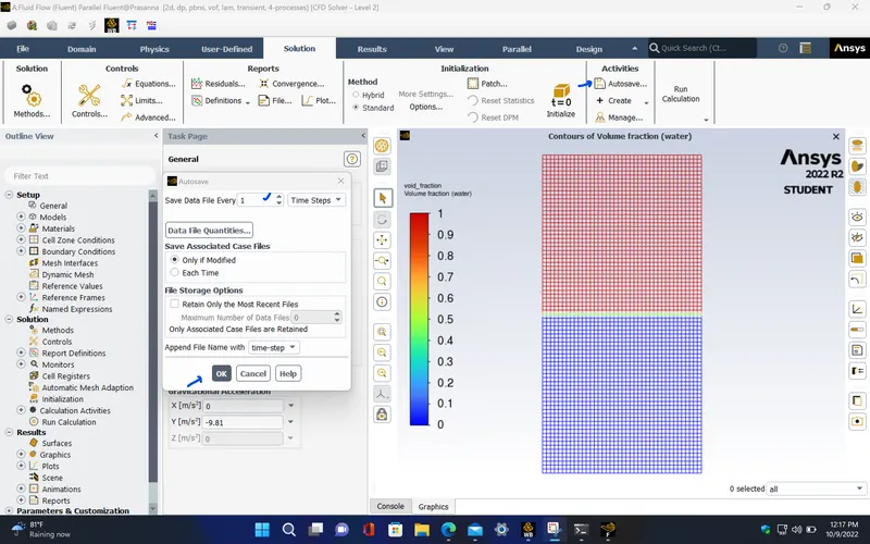
- To create animation in post processing, use autosave option for saving each timestep data.
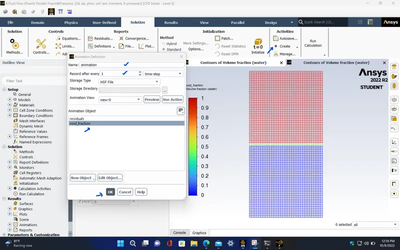
- To create animation in fluent window itself, click create under activities and select the solution animation option from it. Now, select the required timestep frame for recording and animation object as the contour that we have created before.
- Here, we run the simulation for 10 flow seconds which will be more than enough for these fluids to get settled. So, we choose time step size as 0.01 and number of time steps to be 1000 which will give us 10 flow seconds if we multiply those two values.
|
Unsteady Calculation Parameters |
|
|
Number of Time Steps |
1000 |
|
Time Step Size [s] |
0.01 |
|
Max Iterations/Time Step |
20 |
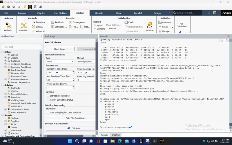
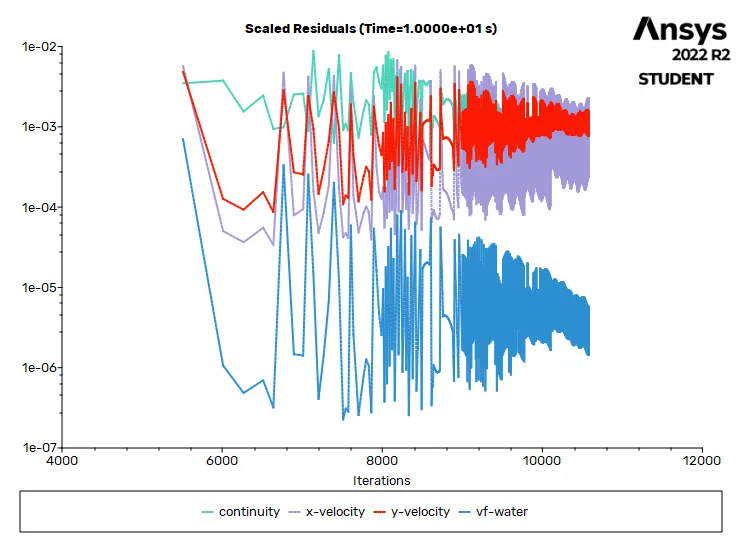
RESIDUAL PLOTS :
Report definitions :
|
delta-time |
0.01 |
s |
|
flow-time |
10 |
s |
CASE - 2 (Water and Air, Mesh element size as 0.3 mm) :
PRE-PROCESSING :
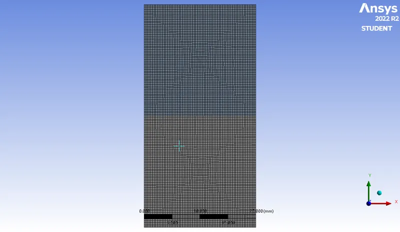
- Here, change the mesh element size to 0.3 mm and repeat all the steps followed as before.
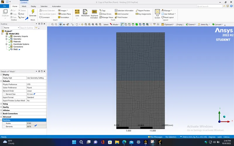
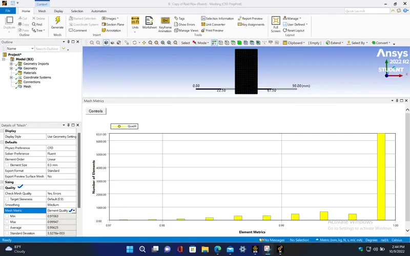
|
Cells |
Faces |
Nodes |
|
8978 |
18157 |
9180 |
SETUP AND SOLVING :
- Setup the problem by selecting the multiphase solver and volume of fluid method for this simulation. The parameters which are chosen are as follows,
|
Model |
Settings |
|
Space |
2D |
|
Time |
Unsteady, 1st-Order Implicit |
|
Model |
Settings |
|
Viscous |
Laminar |
|
Multiphase |
Volume of Fluid |
Materials properties :
|
Fluid |
water-liquid |
|
Density |
998.2 kg/m^3 |
|
Cp (Specific Heat) |
4182 J/(kg K) |
|
Thermal Conductivity |
0.6 W/(m K) |
|
Viscosity |
0.001003 kg/(m s) |
|
Molecular Weight |
18.0152 kg/kmol |
|
Fluid |
air |
|
Density |
1.225 kg/m^3 |
|
Cp (Specific Heat) |
1006.43 J/(kg K) |
|
Thermal Conductivity |
0.0242 W/(m K) |
|
Viscosity |
1.7894e-05 kg/(m s) |
|
Molecular Weight |
28.966 kg/kmol |
Solver :
|
Pressure-Velocity Coupling |
SIMPLE |
- Here, we run the simulation for 10 flow seconds which will be more than enough for these fluids to get settled. So, we choose time step size as 0.01 and number of time steps to be 1000 which will give us 10 flow seconds if we multiply those two values.
RESIDUAL PLOTS :
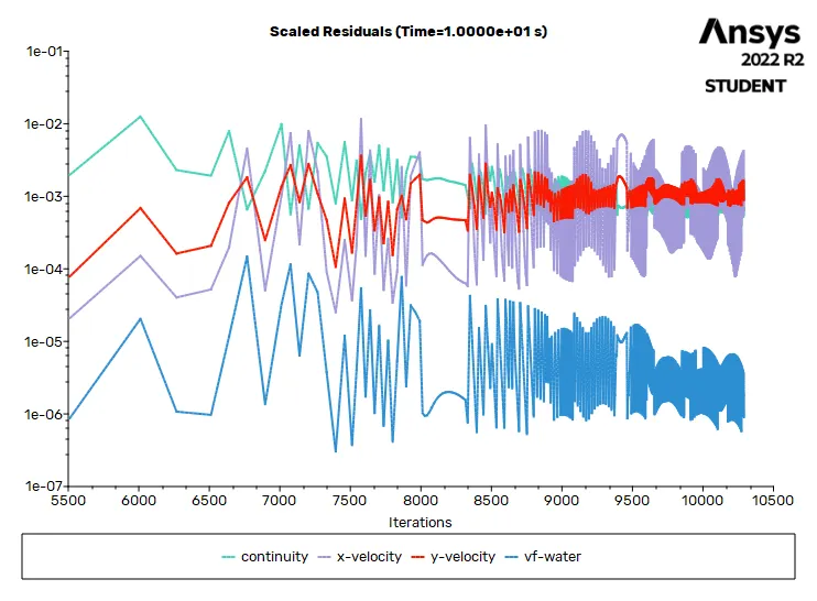
|
Unsteady Calculation Parameters |
|
|
Number of Time Steps |
1000 |
|
Time Step Size [s] |
0.01 |
|
Max Iterations/Time Step |
20 |
Report definitions :
|
delta-time |
0.01 |
s |
|
flow-time |
10 |
s |
CASE - 3 (Water and Air, Mesh element size as 0.1 mm) :
PRE-PROCESSING :
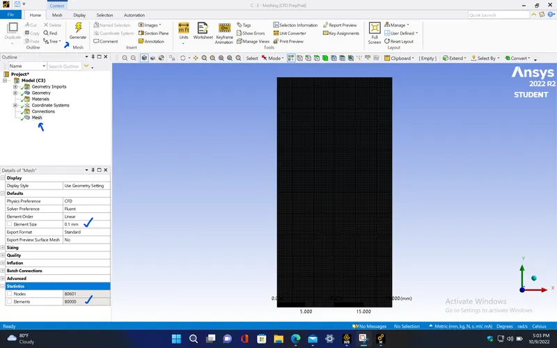
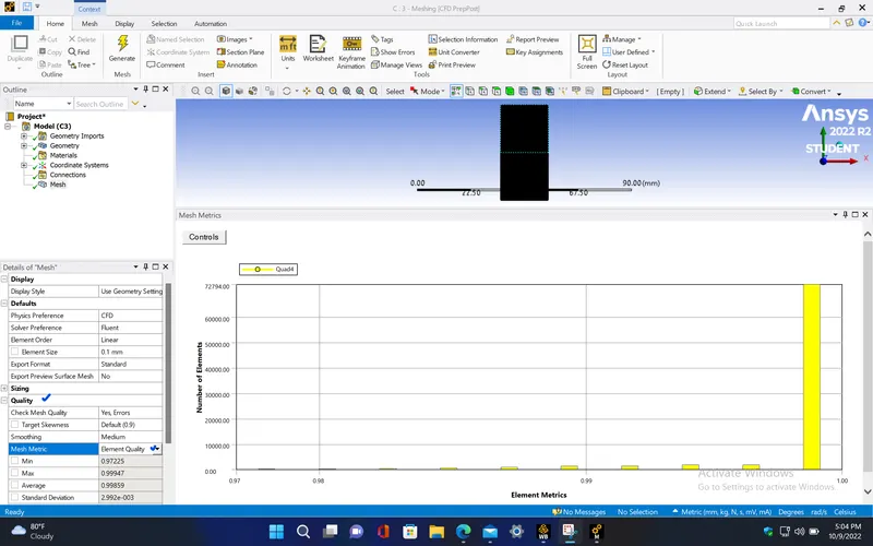
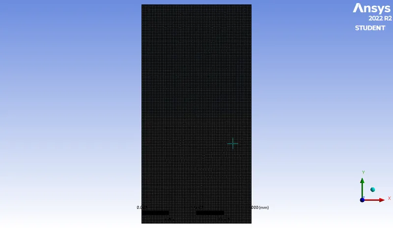
- Here, change the mesh element size to 0.1 mm and generate the mesh. Then, repeat the same steps as discussed before.
|
Cells |
Faces |
Nodes |
|
80000 |
160600 |
80601 |
SETUP AND SOLVING :
- Setup the problem by selecting the multiphase solver and volume of fluid method for this simulation. The parameters which are chosen are as follows,
|
Model |
Settings |
|
Space |
2D |
|
Time |
Unsteady, 1st-Order Implicit |
|
Viscous |
Laminar |
|
Multiphase |
Volume of Fluid |
Material properties :
|
Fluid |
water-liquid |
|
Density |
998.2 kg/m^3 |
|
Cp (Specific Heat) |
4182 J/(kg K) |
|
Thermal Conductivity |
0.6 W/(m K) |
|
Viscosity |
0.001003 kg/(m s) |
|
Molecular Weight |
18.0152 kg/kmol |
|
Fluid |
air |
|
Density |
1.225 kg/m^3 |
|
Cp (Specific Heat) |
1006.43 J/(kg K) |
|
Thermal Conductivity |
0.0242 W/(m K) |
|
Viscosity |
1.7894e-05 kg/(m s) |
|
Molecular Weight |
28.966 kg/kmol |
Solver :
|
Pressure-Velocity Coupling |
SIMPLE |
- Here, we run the simulation for 5 flow seconds since the mesh element size is higher, it will take more computational time than previous cases. Also 5 flow seconds will be more than sufficient for these fluids to get settled.
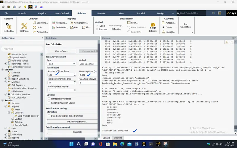
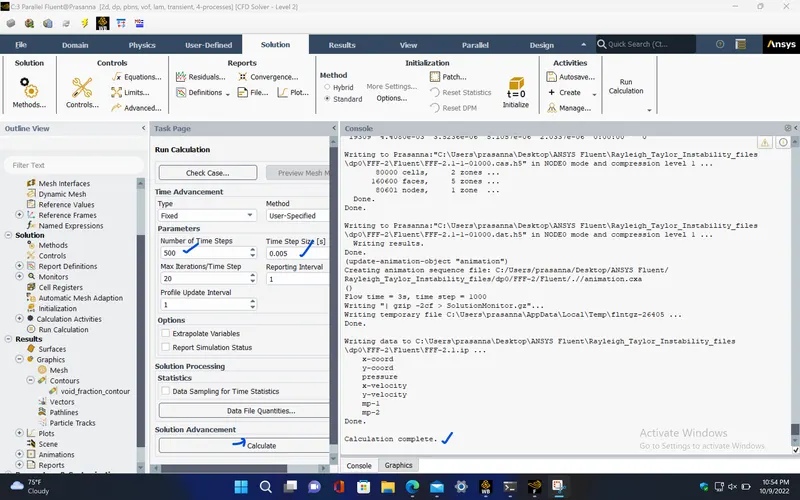
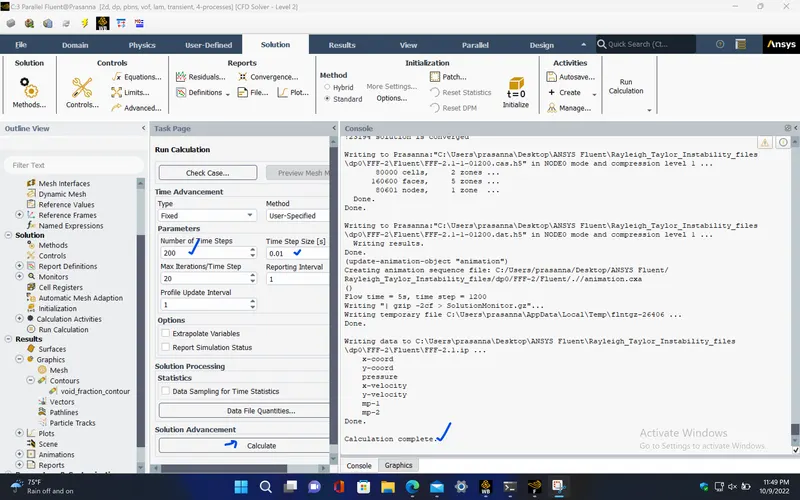
- Unlike in previous cases where we used only a single time step size for the entire simulation, here, we are going to change the time step size for required interval of time. This is done in order to avoid the floating point exception error. So, for first 500 number of time steps, 0.001 can be given as the time step size and this gives the simulation flow time of 0.5 seconds. Then, for next 500 number of time steps, 0.005 can be given as the step size and this gives the flow time of 2.5 seconds. Finally, for the last 200 number of time steps, 0.01 is given as the time step size and this gives 2 flow seconds. So, in total, the simulation ran for 5 flow seconds.
|
Unsteady Calculation Parameters |
|
|
Number of Time Steps |
500 |
|
Time Step Size [s] |
0.001 |
|
Max Iterations/Time Step |
20 |
|
Unsteady Calculation Parameters |
|
|
Number of Time Steps |
500 |
|
Time Step Size [s] |
0.005 |
|
Max Iterations/Time Step |
20 |
|
Unsteady Calculation Parameters |
|
|
Number of Time Steps |
200 |
|
Time Step Size [s] |
0.01 |
|
Max Iterations/Time Step |
20 |
RESIDUAL PLOTS :
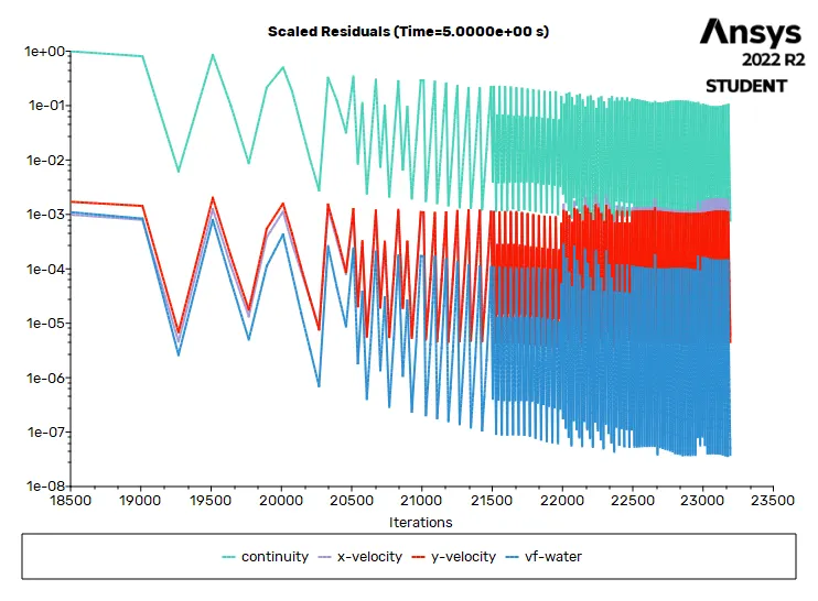
Solution status :
|
Value |
Absolute Criteria |
Convergence Status |
|
|
continuity |
0.0007501077 |
0.001 |
Converged |
|
x-velocity |
6.231166e-06 |
0.001 |
Converged |
|
y-velocity |
4.468475e-06 |
0.001 |
Converged |
|
vf-water |
3.493263e-08 |
0.001 |
Converged |
Report definitions :
|
delta-time |
0.01 |
s |
|
iters-per-timestep |
0 |
|
|
flow-time |
5 |
s |
CASE - 4 (Water and User defined fluid, Mesh element size as 0.1 mm) :
- Here, change the mesh element size to 0.1 mm and generate the mesh. Then, repeat the same steps as discussed before.
|
Cells |
Faces |
Nodes |
|
80000 |
160600 |
80601 |
SETUP AND SOLVING :
- Setup the problem by selecting the multiphase solver and volume of fluid method for this simulation. The parameters which are chosen are as follows,
|
Model |
Settings |
|
Space |
2D |
|
Time |
Unsteady, 1st-Order Implicit |
|
Viscous |
Laminar |
|
Multiphase |
Volume of Fluid |
Material properties :
|
Fluid |
water-liquid |
|
Density |
998.2 kg/m^3 |
|
Cp (Specific Heat) |
4182 J/(kg K) |
|
Thermal Conductivity |
0.6 W/(m K) |
|
Viscosity |
0.001003 kg/(m s) |
|
Molecular Weight |
18.0152 kg/kmol |
|
Fluid |
user_defined_fluid |
|
Density |
400 kg/m^3 |
|
Cp (Specific Heat) |
1006.43 J/(kg K) |
|
Thermal Conductivity |
0.0242 W/(m K) |
|
Viscosity |
0.001 kg/(m s) |
|
Molecular Weight |
28.966 kg/kmol |
Solver :
|
Pressure-Velocity Coupling |
SIMPLE |
- Here, change the air properties with density as 400 kg/m^3 and viscosity as 0.001 kg/m-s and rename it as user defined fluid.
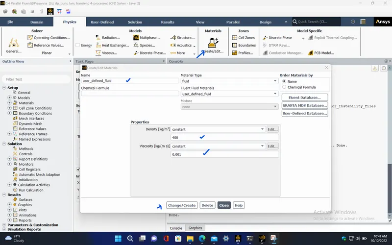
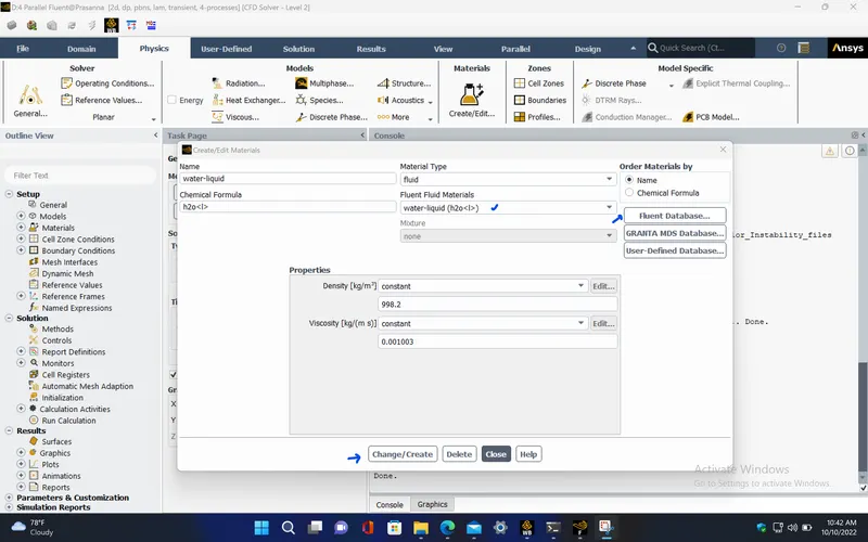
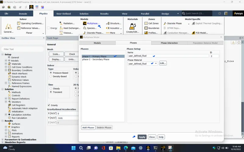
- Now, select the primary phase as user defined fluid and secondary phase as water.
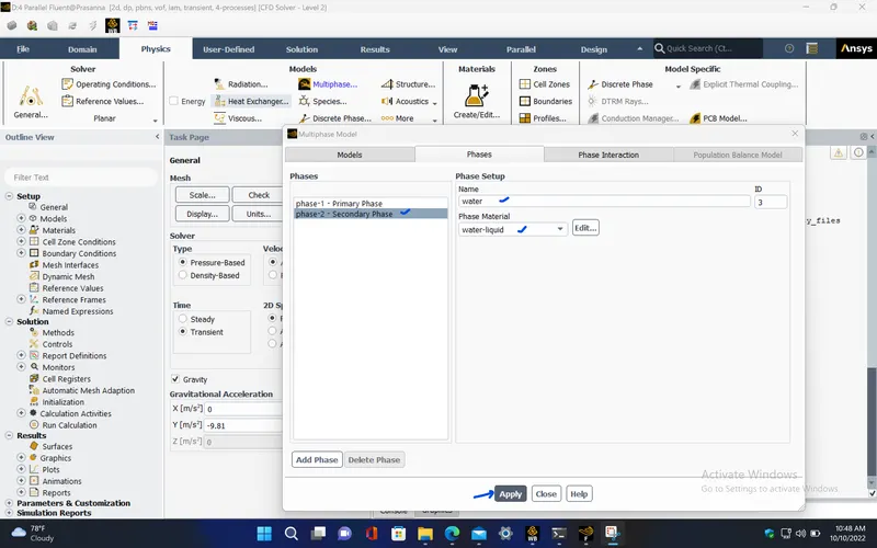
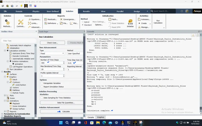
- Here, we run the simulation for 7 flow seconds, since the user defined fluid has the higher density than air, fluids will take some more time than the previous case to get settled.
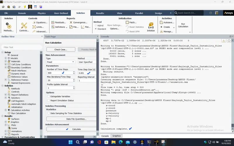
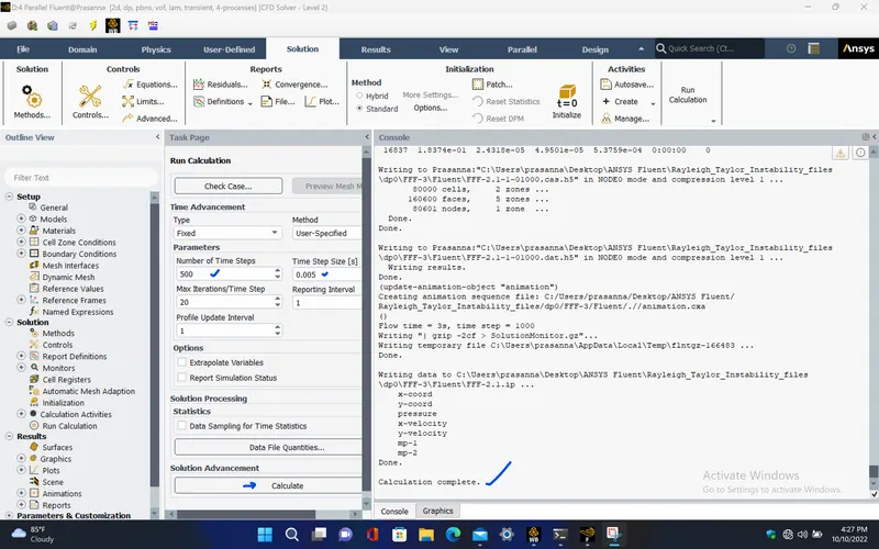
- Here also, we are going to change the time step size for required intervals of time. This is done in order to avoid the floating point exception error. So, for first 500 number of time steps, 0.001 can be given as the time step size and this gives the simulation flow time of 0.5 seconds. Then, for next 500 number of time steps, 0.005 can be given as the step size and this gives the flow time of 2.5 seconds. Finally, for the last 400 number of time steps, 0.01 is given as the time step size and this gives 4 flow seconds. So, in total, the simulation ran for 7 flow seconds.
|
Unsteady Calculation Parameters |
|
|
Number of Time Steps |
500 |
|
Time Step Size [s] |
0.001 |
|
Max Iterations/Time Step |
20 |
|
Unsteady Calculation Parameters |
|
|
Number of Time Steps |
500 |
|
Time Step Size [s] |
0.005 |
|
Max Iterations/Time Step |
20 |
|
Unsteady Calculation Parameters |
|
|
Number of Time Steps |
400 |
|
Time Step Size [s] |
0.01 |
|
Max Iterations/Time Step |
20 |
RESIDUALS PLOT :
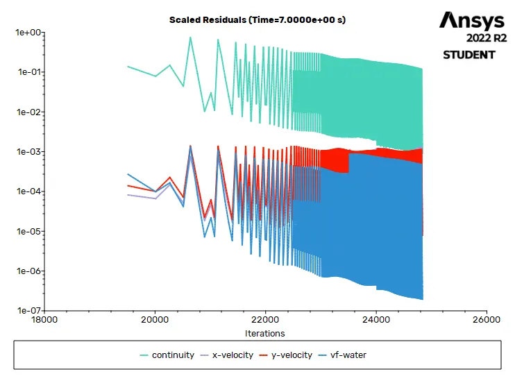
Solution status :
|
Value |
Absolute Criteria |
Convergence Status |
|
|
continuity |
0.0009007384 |
0.001 |
Converged |
|
x-velocity |
1.083585e-05 |
0.001 |
Converged |
|
y-velocity |
7.872593e-06 |
0.001 |
Converged |
|
vf-water |
1.954481e-07 |
0.001 |
Converged |
Report definitions :
|
delta-time |
0.01 |
s |
|
flow-time |
7 |
s |
RESULTS :
Animations (Google drive links) :
For Case 1,
https://drive.google.com/file/d/1LgkUpD6qfCm7rvsT-_Lfnitod60LrQpl/view?usp=sharing
For Case 2,
https://drive.google.com/file/d/1xhldeQqnIksJiRlH6ZbzFAOtGP5Llo48/view?usp=sharing
For Case 3,
https://drive.google.com/file/d/1UxCel86JiNbRWimcShVMh9W8820fvDHV/view?usp=sharing
For Case 4,
https://drive.google.com/file/d/1ZknpMxzOGfHWg_KQjJH5srucFAy1w2md/view?usp=sharing
MESH INDEPENDENCY STUDY :
|
FLUIDS |
MESH ELEMENT SIZE (in 'mm') |
NUMBER OF MESH ELEMENTS |
ATWOOD NUMBER |
|
|
CASE - 1 |
Water and Air |
0.5 |
3200 |
0.9975 |
|
CASE - 2 |
Water and Air |
0.3 |
8978 |
|
|
CASE - 3 |
Water and Air |
0.1 (Refined) |
80000 |
|
|
CASE - 4 |
Water and User defined fluid |
0.1 (Refined) |
80000 |
0.4278 |
CONCLUSION :
From the animations for the first three cases of different mesh element size, we can observe that, the Rayleigh instability is captured more accurately in the case which has the finer mesh size(0.1 mm). So, we can say that, As we decrease the mesh element size, the even smaller volumes of the fluids can be captured properly, but in contrast, it will also take more computational time running the simulation. Therefore, the most optimum mesh element size has to be selected. Here, Case-3 with 0.1 mesh element size was chosen since the number of mesh elements was not so huge.
For case-4 for Rayleigh instability simulation of water and user defined fluid, 0.1 mm mesh size was chosen. Also, from the above table, we can observe that the case with water and air as the fluids, the Atwood number is found to be 0.9975 whereas for water and user defined fluid, it is 0.4278. This tells that, As the difference in densities of the two immiscible fluids increases, the Atwood number also increases which results in higher and faster penetration distance of water into the air.