Challenge

Week 4.1 - Genetic Algorithm

AIM :

To find the global maxima for the stalagmite function using ga and to plot the results.

MAIN PROGRAM :

% To find the global maxima for the stalagmite function using ga and plot the results

clear all
close all
clc

% Defining the search space
x = linspace(0,0.6,150);
y = linspace(0,0.6,150);

% Creating 2 Dimensional array mesh
[xx, yy] = meshgrid(x,y);

% Preallocating the variables which are inside the loop
f = zeros(150,150);
fopt1 = zeros(1,50);
fopt2 = zeros(1,50);
fopt3 = zeros(1,50);
xopt1 = zeros(1,50);
xopt2 = zeros(1,50);
xopt3 = zeros(1,50);
yopt1 = zeros(1,50);
yopt2 = zeros(1,50);
yopt3 = zeros(1,50);

% Creating the stalagmite function
for i = 1 : length(xx)
    for j = 1 : length(yy)
        input_vector(1) = xx(i,j);
        input_vector(2) = yy(i,j);
        f(i,j) = stalagmite(input_vector);
    end
end

F = -f;

% Number of iterations
num_cases = 50;

% Case study 1, finding the global maxima using ga without the input bounds

tic

for i = 1 : num_cases

    [inputs1, fopt1(i)] = ga(@stalagmite, 2);

    xopt1(i) = inputs1(1);
    yopt1(i) = inputs1(2);

end

Fopt1 = -fopt1;

% Time taken for case study 1 ( in seconds)
study_time1 = toc

% Plotting for case study 1

figure(1)
subplot(2,1,1)
hold on
surfc(xx,yy,F)
shading interp
xlabel('x value')
ylabel('y value')
zlabel('Function (F)')
plot3(xopt1,yopt1,Fopt1,'marker','o',MarkerSize=5,MarkerFaceColor='r')
title('Unbounded inputs')
subplot(2,1,2)
plot(Fopt1)
xlabel('Iterations')
ylabel('Function - Maximum')
hold off


% Case study 2, finding the global maxima using ga with the bounded inputs.

tic

for i = 1 : num_cases

    [inputs2, fopt2(i)] = ga(@stalagmite, 2, [],[],[],[],[0;0],[0.6;0.6]);

    xopt2(i) = inputs2(1);
    yopt2(i) = inputs2(2);

end

Fopt2 = -fopt2;

% Time taken for case study 2 ( in seconds)
study_time2 = toc

% Plotting for case study 2

figure(2)
subplot(2,1,1)
hold on
surfc(xx,yy,F)
shading interp
xlabel('x value')
ylabel('y value')
zlabel('Function (F)')
plot3(xopt2,yopt2,Fopt2,'marker','o',MarkerSize=5,MarkerFaceColor='r')
title('Bounded inputs')
subplot(2,1,2)
plot(Fopt2)
xlabel('Iterations')
ylabel('Function - Maximum')
hold off


% Case study 3, finding the global maxima using ga with the input bounds and modified initial population

options = optimoptions('ga');
options = optimoptions(options,'PopulationSize',250);

tic

for i = 1 : num_cases

    [inputs3, fopt3(i)] = ga(@stalagmite,2,[],[],[],[],[0;0],[0.6;0.6],[],[],options);

    xopt3(i) = inputs3(1);
    yopt3(i) = inputs3(2);

end

Fopt3 = -fopt3;

Fmax = mean(Fopt3)

% Time taken for case study 3 ( in seconds)
study_time3 = toc

% Global maxima of the stalagmite funtion

Global_maxima = table(inputs3,Fmax)


% Plotting for case study 3

figure(3)
subplot(2,1,1)
hold on
surfc(xx,yy,F)
shading interp
xlabel('x value')
ylabel('y value')
zlabel('Function (F)')
plot3(xopt3,yopt3,Fopt3,'marker','o',MarkerSize=5,MarkerFaceColor='r')
title('Bounded inputs with modified population size')
subplot(2,1,2)
plot(Fopt3)
xlabel('Iterations')
ylabel('Function - Maximum')
hold off

FUNCTION PROGRAM :

% To find the stalagmite function

function S = stalagmite(F)

f1 = (sin((5.1*pi*F(1))+0.5))^6;
f2 = (sin((5.1*pi*F(2))+0.5))^6;
f3 = exp(-4*log(2)*( ((F(1)-0.0667)^2) / 0.64 ) );
f4 = exp(-4 * log(2) * ( ((F(2)-0.0667)^2) / 0.64 ) );

S = -(f1*f2*f3*f4);

end

OUTPUT PLOTS :

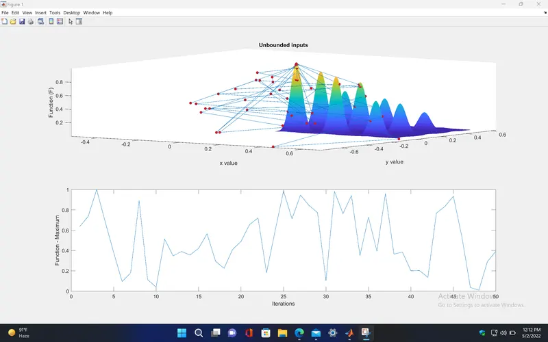
Case study 1 : Unbounded inputs for ga
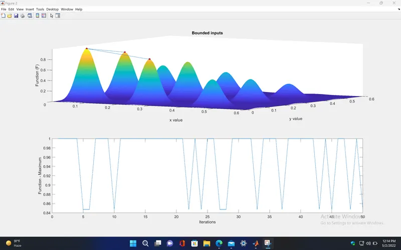
Case study 2 : Bounded inputs for ga
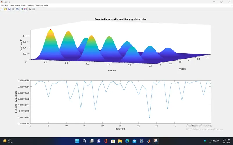
Case study 3 : Bounded inputs with modified initial population for ga
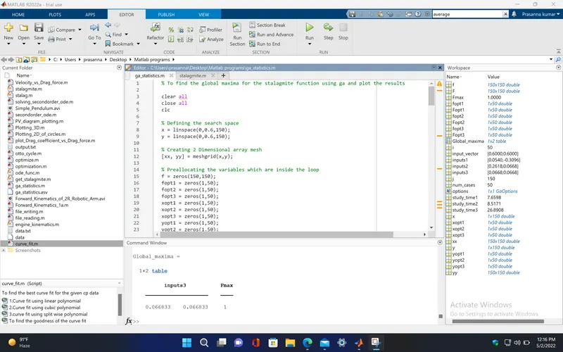
Output in command window,
EXPLANATION :

Optimization :

It a method for finding a optimum or near optimum solution by comparing various solutions of the function under a given set of constraints.

Genetic algorithm :

It is algorithm based on the evolutionary theory. It can be used to find a best solution from various solutions of the optimization problem within the given constraints. The steps involved in genetic algorithm are as follows.

  • Initialization
  • Selection
  • Crossover
  • Mutation

Initialization :

  • Here,the population size is given for the function to initialize the algorithm. Higher the population size, more accurate the solution since it will take a range of values for evaluating the fitness function.
  • Fitness function which is also known as the objective function is a mathematical model which takes in the desired inputs to provide the output required for the problem.

Selection :

  • Then, the best solutions are selected by using roulette wheel selection method. Here, the roulette wheel is rotated, which has a fixed point and for each time wheel is rotated, the fixed point indicates the solution to be selected. The wheel is made such a way that, the solution with higher fitness value will have greater pie.

Crossover :

  • Here, the next generation solution (also referred as child) is formed by interchanging some values from two of the selected solutions (referred to parents) by a single point or double point cross over technique. It is used to converge various solutions to find the best one.

Mutation :

  • Sometimes, due to cross overs, the solution may get to stuck within the local minima or maxima. So, inorder to avoid this and to find the global solution, the solutions are made diversed by changing any value in the solution randomly which is known as mutation.

Termination or stopping criteria :

  • The 'ga' should have a stopping criteria inorder to end the algorithm otherwise the 'ga' can run number of times until it gets a single value.
  • The termination statement should be set, with a fixed number of generations or to stop 'ga' if there is a very small or no change in the obtained solution.

Case study :

Since, the 'ga' chooses random values initially, the solution may vary for each time the program run. So, the 'ga' is made to run multiple times inside the loop so that to check the solution obtained changes or not. Based on it, there are three case studies made

  • Case study 1 - Here, the bound input values between which the 'ga' should select the inputs was not provided. So, the 'ga' predicts different solutions when it runs multiple times.
  • Case study 2 - Here, the bound limits are set for the input variables ( between 0 to 0.6 ). Now, the solutions are converged and reduced but some are still indicating the local maximas.
  • Case study 3 - Here, in addition to the bound limits, the population size is modified and set to 250 which by default will be 50. Therefore global maxima is obtained for number of times the 'ga' runs.

Stalagmite function :

  • `f(x,y) = f_1,_x * f_2,_x * f_1,_y * f_2,_y`

Where,

  • `f_1,_x = (sin(5.1*pi*x + 0.5))^6`
  • `f_1,_y = (sin(5.1*pi*y + 0.5))^6`
  • `f_2,_x = exp(-4*ln(2) * ((x - 0.0667)^2 / 0.64))`
  • `f_2,_y = exp(-4*ln(2) * ((y - 0.0667)^2 / 0.64))`

Main code - Explanation:

clear all - Clears all the variables in workspace and also clears the scripts and functions.
close all - Closes all the figure windows.
clc - Clears the command window.
Defining the search space for stalagmite function
x = linspace(0,0.6,150); - Creates a row vector with 150 values between 0 and 0.6, and store the values in variable 'x'.
y = linspace(0,0.6,150); - Creates a row vector with 150 values between 0 and 0.6, and store the values in variable 'y'.
Creating 2 Dimensional array mesh
[xx, yy] = meshgrid(x,y); - Converts the one dimensional row vectors into two dimensional array matrices and store the values in 'xx' and 'yy' respectively.
Preallocating the variables which are inside the loop
f = zeros(150,150); - Creates a 150,150 matrix of zero values and assign it to variable 'f'.
fopt1 = zeros(1,50); - Creates a column vector with 50 zero values and assign it to variable 'fopt1'.
fopt2 = zeros(1,50); - Creates a column vector with 50 zero values and assign it to variable 'fopt2'.
fopt3 = zeros(1,50); - Creates a column vector with 50 zero values and assign it to variable 'fopt3'.
xopt1 = zeros(1,50); - Creates a column vector with 50 zero values and assign it to variable 'xopt1'.
xopt2 = zeros(1,50); - Creates a column vector with 50 zero values and assign it to variable 'xopt2'.
xopt3 = zeros(1,50); - Creates a column vector with 50 zero values and assign it to variable 'xopt3'.
yopt1 = zeros(1,50); - Creates a column vector with 50 zero values and assign it to variable 'yopt1'.
yopt2 = zeros(1,50); - Creates a column vector with 50 zero values and assign it to variable 'yopt2'.
yopt3 = zeros(1,50); - Creates a column vector with 50 zero values and assign it to variable 'yopt3'.
'for' loop is used here for creating the stalagmite function. for every counter value of 'i' and 'j' , the corresponding indices value in 'xx' and 'yy' matrices is passed as input as a row vector to the 'stalagmite' function which calculates and returns a value to create the stalagmite.
for i = 1 : length(xx) - This loop repeats for the incremental counter value from i = 1 to length of 'xx' which is 150.
for j = 1 : length(yy) - This is the nested for loop. for every counter value of 'i', the counter value 'j' increments until the length of 'yy' which is 150.
input_vector(1) = xx(i,j); - for every time the loop runs, the corresponding indices value of 'i' and 'j' in the matrix 'xx' is set to the first value of 'input_vector'.
input_vector(2) = yy(i,j); - for every time the loop runs, the corresponding indices value of 'i' and 'j' in the matrix 'yy' is set to the second value of 'input_vector'.
f(i,j) = stalagmite(input_vector); - The 'stalagmite' function takes the values of the 'input_vector' as input and returns the output which is stored in the variable 'f' for the corresponding indices value of 'i' and 'j' of the loop.
end - Ends the nested loop.
end - Ends the loop.
F = -f; - The calculated stalagmite function 'f' is given a negative sign and set to a variable 'F' , which is to get a positive peak(maximum) in the plot.
Number of iterations
num_cases = 50; - Number of iterations for 'ga' is set to 50 which is assigned to the variable 'num_cases'.
Case study 1, finding the global maxima using ga without the input bounds
tic - Saves the current time, Start of the timer.
'for' loop is used here to run the 'ga' command for the 50 iterations to check if the 'ga' predicts the same value for every iterations.
for i = 1 : num_cases - Runs the loop 50 times.
[inputs1, fopt1(i)] = ga(@stalagmite, 2); - Finds the minimum of the function where the inputs given to the 'ga' are
  • the '@stalagmite', is the objective function which 'ga' uses to find the best fitness value and it is initiated with a function handle ' @',
  • the number of input variables(i.e,'2') for the function which 'ga' changes (initially, the 'ga' chooses these values randomly and since, there is no bound limits given to 'ga', it chooses from a wide range of values).
  • Then, the 'ga' calculates and returns two outputs where one is a row vector containing the values of the inputs of which the function is minimum and stores it in the variable 'inputs1' and the other is a column vector of values of the fitness function over 50 iterations of the loop and it is stored in the variable 'fopt1' for each iteration of the loop.
xopt1(i) = inputs1(1); - For each iteration of the loop defined by the variable 'i', the first value of the row vector named 'inputs1' is assigned to the variable 'xopt1' which forms a column vector of values, arranged with a respective position defined by 'i'.
yopt1(i) = inputs1(2); - For each iteration of the loop defined by the variable 'i', the second value of the row vector named 'inputs1' is assigned to the variable 'yopt1' which forms a column vector of values, arranged with a respective position defined by 'i'.
end - End of the loop.
Fopt1 = -fopt1; - The calculated stalagmite function 'fopt1' is given a negative sign and set to a variable 'Fopt1' , which is to get a positive peak(maximum) in the plot.
Time taken for case study 1 ( in seconds)
study_time1 = toc - Calculates the elapsed time(in seconds) from the recorded value and stores the value in the variable 'study_time1'. Stops the timer.
Plotting for case study 1
figure(1) - Creates the figure window named 'Figure 1'.
subplot(2,1,1) - Creates the subplot in the 'Figure 1' window. This command divides the current figure window into 2 rows and 1 column , positions the plot in the first row.
hold on - Holds the same figure window for multiple plotting.
surfc(xx,yy,F) - Creates a three dimensional surface plot with contour plot.
shading interp - Removes the grid lines created by 'surfc' command.
xlabel('x value') - Labels x-axis as 'x value' in the surface plot.
ylabel('y value') - Labels y-axis as 'y value' in the surface plot.
zlabel('Function (F)') - Labels z-axis as 'Function (F)' in the surface plot.
plot3(xopt1,yopt1,Fopt1,'marker','o',MarkerSize=5,MarkerFaceColor='r') - Plots in the three dimensional space using the co-ordinates '(xopt1,yopt1,zopt1)' with marker size as 5 and marker face colour as red.
title('Unbounded inputs') - Names the title of the plot as 'Unbounded inputs'.
subplot(2,1,2) - Creates the second subplot in the second row position of the same figure window.
plot(Fopt1) - Plots 'Fopt1' for number of iterations which is 50.
xlabel('Iterations') - Labels x-axis as 'Iterations' in the second subplot.
ylabel('Function - Maximum') - Labels y-axis as 'Function - Maximum' in the second subplot.
hold off - Sets the 'hold' command to off for this figure window.
Case study 2, finding the global maxima using ga with the bounded inputs.
tic - Saves the current time, Start of the timer.
for i = 1 : num_cases - Runs the loop 50 times.
[inputs2, fopt2(i)] = ga(@stalagmite, 2, [],[],[],[],[0;0],[0.6;0.6]); - Finds the minimum of the function where the inputs given to the 'ga' are,
  • the '@stalagmite', is the objective function which 'ga' uses to find the best fitness value and it is initiated with a function handle ' @',
  • the number of input variables(i.e,'2') for the function which 'ga' changes to find the optimum solution,
  • the first and second set of square brackets '[], []' are empty since there is no linear inequalities given as a constrain for the function. If there is any linear inequalities given for the function, then, 'ga' uses this inequality constraints to find the value within the default tolerence value of '1*e-3' ,
  • the third and fourth set of square brackets '[], []' are empty since there is no linear equalities given as a constrain to the function. If there is any linear equalities given for the function, then, 'ga' uses this equality constraints to find the value within the default tolerence value of '1*e-3' ,
  • [0;0],[0.6;0.6] ' are the lower and upper bounds for the stalagmite function. Here, 'ga' chooses the input values between these bounded values and finds the global minimum of the function but here it is the global maximum of the function since the function is given a negative sign ( ' -ve ' ).
  • Then, the 'ga' calculates and returns two outputs where one is a row vector containing the values of the inputs of which the function is minimum and stores it in the variable 'inputs2' and the other is a column vector of values of the fitness function over 50 iterations of the loop and it is stored in the variable 'fopt2' for each iteration of the loop.
xopt2(i) = inputs2(1); - For each iteration of the loop defined by the variable 'i', the first value of the row vector named 'inputs2' is assigned to the variable 'xopt2' which forms a column vector of values, arranged with a respective position defined by 'i'.
yopt2(i) = inputs2(2); - For each iteration of the loop defined by the variable 'i', the second value of the row vector named 'inputs2' is assigned to the variable 'yopt2' which forms a column vector of values, arranged with a respective position defined by 'i'.
end - End of the loop.
Fopt2 = -fopt2; - The calculated stalagmite function 'fopt2' is given a negative sign and set to a variable 'Fopt2' , which is to get a positive peak(maximum) in the plot.
Time taken for case study 2 ( in seconds)
study_time2 = toc - Calculates the elapsed time(in seconds) from the recorded value and stores the value in the variable 'study_time2'. Stops the timer.
Plotting for case study 2
figure(2) - Creates the figure window named 'Figure 2'.
subplot(2,1,1) - Creates the subplot in the 'Figure 2' window. This command divides the current figure window into 2 rows and 1 column , positions the plot in the first row.
hold on - Holds the same figure window for multiple plotting.
surfc(xx,yy,F) - Creates a three dimensional surface plot with contour plot.
shading interp - Removes the grid lines created by 'surfc' command.
xlabel('x value') - Labels x-axis as 'x value' in the surface plot.
ylabel('y value') - Labels y-axis as 'y value' in the surface plot.
zlabel('Function (F)') - Labels z-axis as 'Function (F)' in the surface plot.
plot3(xopt2,yopt2,Fopt2,'marker','o',MarkerSize=5,MarkerFaceColor='r') - Plots in the three dimensional space using the co-ordinates '(xopt2,yopt2,zopt2)' with marker size as 5 and marker face colour as red.
title('Bounded inputs') - Names the title of the plot as 'Bounded inputs'.
subplot(2,1,2) - Creates the second subplot in the second row position of the same figure window.
plot(Fopt2) - Plots 'Fopt2' for number of iterations which is 50.
xlabel('Iterations') - Labels x-axis as 'Iterations' in the second subplot.
ylabel('Function - Maximum') - Labels y-axis as 'Function - Maximum' in the second subplot.
hold off - Sets the 'hold' command to off for this figure window.
Case study 3, finding the global maxima using ga with the input bounds and modified initial population.
options = optimoptions('ga', 'PopulationSize', 250); - The population size, the 'ga' takes, is set to '250' by using the command 'optimoptions' which takes the inputs such as 'solver','name',value which is in here 'ga', 'PopulationSize', 250 respectively. By default, the population size is 50 and this is not enough to find the global maxima of the function, as the function also has local maximas. Inorder to find the global maxima of the function, the population size is increased so that the 'ga' initiates with larger population size.
tic - Saves the current time, Start of the timer.
for i = 1 : num_cases - Runs the loop 50 times.
[inputs3, fopt3(i)] = ga(@stalagmite,2,[],[],[],[],[0;0],[0.6;0.6],[],[],options); - Finds the minimum of the function where the inputs given to the 'ga' are,
  • the '@stalagmite', is the objective function which 'ga' uses to find the best fitness value and it is initiated with a function handle ' @',
  • the number of input variables(i.e,'2') for the function which 'ga' changes to find the optimum solution,
  • the first and second set of square brackets '[], []' are empty since there is no linear inequalities given as a constrain for the function. If there is any linear inequalities given for the function, then, 'ga' uses this inequality constraints to find the value within the default tolerance value of '1*e-3' ,
  • the third and fourth set of square brackets '[], []' are empty since there is no linear equalities given as a constrain to the function. If there is any linear equalities given for the function, then, 'ga' uses this equality constraints to find the value within the default tolerance value of '1*e-3' ,
  • [0;0],[0.6;0.6] ' are the lower and upper bounds for the stalagmite function. Here, 'ga' chooses the input values between these bounded values and finds the global minimum of the function but here it is the global maximum of the function since the function is given a negative sign ( ' -ve ' ),
  • the next square brackets '[]' is set as empty since there is no non-linear equality and inequality constraints for the function and if it has any, then, 'ga' uses these non-linear constraints to find the minimum value of the function and the value of the non-linear inequality and equality will be satisfied within the default tolerance value of '1*e-3'.
  • the last square bracket '[]' is set as empty since there is no specific variables which is given to take only integer values. If this integer constraint is to be set, then, 'ga' accepts only non-linear inequality contraints and not the non-linear equality constraints,
  • options' is set to have a modified parameter values for 'ga'.
  • Then, the 'ga' calculates and returns two outputs where one is a row vector containing the values of the inputs of which the function is minimum and stores it in the variable 'inputs2' and the other is a column vector of values of the fitness function over 50 iterations of the loop and it is stored in the variable 'fopt2' for each iteration of the loop.
xopt3(i) = inputs3(1); - For each iteration of the loop defined by the variable 'i', the first value of the row vector named 'inputs3' is assigned to the variable 'xopt3' which forms a column vector of values, arranged with a respective position defined by 'i'.
yopt3(i) = inputs3(2); - For each iteration of the loop defined by the variable 'i', the second value of the row vector named 'inputs3' is assigned to the variable 'yopt3' which forms a column vector of values, arranged with a respective position defined by 'i'.
end - End of the loop.
Fopt3 = -fopt3; - The calculated stalagmite function 'fopt3' is given a negative sign and set to a variable 'Fopt3' , which is to get a positive peaks(maximum) in the plot.
Fmax = mean(Fopt3) - Finds the mean of 'Fopt3'.
Time taken for case study 3 ( in seconds)
study_time3 = toc - Calculates the elapsed time(in seconds) from the recorded value and stores the value in the variable 'study_time3'. Stops the timer.
Global maxima of the stalagmite funtion
Global_maxima = table(inputs3,Fmax)
Plotting for case study 3
figure(3) - Creates the figure window named 'Figure 3'.
subplot(2,1,1) - Creates the subplot in the 'Figure 3' window. This command divides the current figure window into 2 rows and 1 column , positions the plot in the first row.
hold on - Holds the same figure window for multiple plotting.
surfc(xx,yy,F) - Creates a three dimensional surface plot with contour plot.
shading interp - Removes the grid lines created by 'surfc' command.
xlabel('x value') - Labels x-axis as 'x value' in the surface plot.
ylabel('y value') - Labels y-axis as 'y value' in the surface plot.
zlabel('Function (F)') - Labels z-axis as 'Function (F)' in the surface plot.
plot3(xopt3,yopt3,Fopt3,'marker','o',MarkerSize=5,MarkerFaceColor='r') - Plots in the three dimensional space using the co-ordinates '(xopt3,yopt3,zopt3)' with marker size as 5 and marker face colour as red.
title('Bounded inputs with modified population size') - Names the title of the plot as 'Bounded inputs with modified population size'.
subplot(2,1,2) - Creates the second subplot in the second row position of the same figure window.
plot(Fopt3) - Plots 'Fopt3' for number of iterations which is 50.
xlabel('Iterations') - Labels x-axis as 'Iterations' in the second subplot.
ylabel('Function - Maximum') - Labels y-axis as 'Function - Maximum' in the second subplot.
hold off - Sets the 'hold' command to off for this figure window.
Function code - Explanation :
Calculating the stalagmite function, for every time the loop inside the main code runs , the function code returns the output.
function S = stalagmite(F) - Creates a function named 'stalagmite'
f1 = (sin((5.1*pi*F(1))+0.5))^6;
f2 = (sin((5.1*pi*F(2))+0.5))^6;
f3 = exp(-4*log(2)*( ((F(1)-0.0667)^2) / 0.64 ) );
f4 = exp(-4 * log(2) * ( ((F(2)-0.0667)^2) / 0.64 ) );
S = -(f1*f2*f3*f4); - Negative sign indicates that the function is inverted. Since, the 'ga' command in matlab can find only the minimum of the function inorder to find the maximum, the function is inverted.
end - Ends the function code.
RESULT :
  • The global maxima of the stalagmite function found by using 'ga' is 0.99999 approximately equal to 1 of which the inputs are [ 0.0668 0.0668 ] .
ERRORS OCCURED WHILE PROGRAMMING :
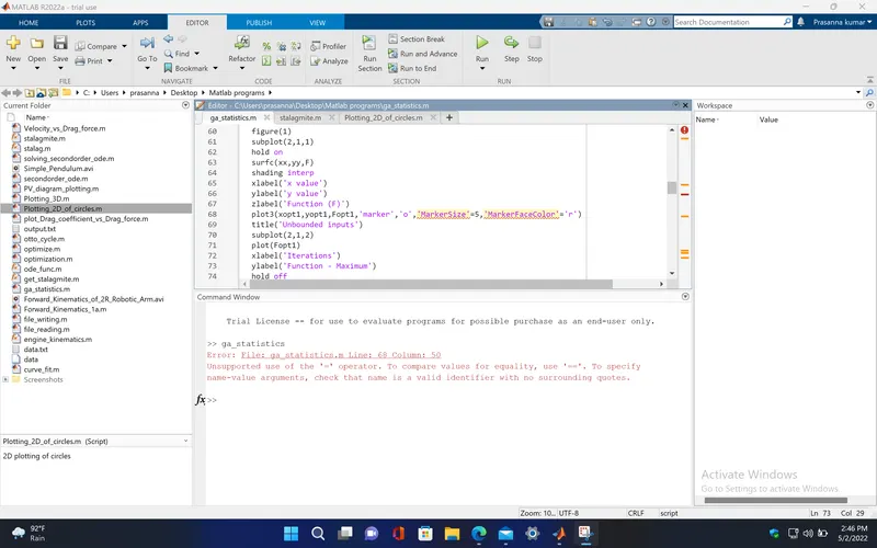
  • Inside the 'plot3' command, I have used the 'MarkerSize'=5 and 'MarkerFaceColor'='r' between the quotation marks which gave me a error when I ran the program.
  • So, I have to delete the quotation marks for MarkerSize=5 and MarkerFaceColor='r' to run the program without error.
REFERENCE :
Your portfolio, next

Ship work like this
in your own course.

Talk to a career counsellor

Free 20-minute call. We'll map the right course to where you want to work.

By submitting you agree to our Terms and Privacy Policy.

Talk to a career counsellor

Free 20-minute call. We'll map the right course to where you want to work.

By submitting you agree to our Terms and Privacy Policy.