Week 3 - Solving second order ODEs

AIM :

To solve the second order ODE of a simple pendulum and animate its motion.

MAIN PROGRAM :

% To solve the second order ODE of a simple pendulum and to animate its motion

clear all
close all
clc

% Input variables

% Mass of the ball(in 'Kg')  
m = 1;
% Acceleration due to gravity(in 'm/s^2')
g = 9.81;
% Length of the pendulum(in 'm')
l = 1;
% Damping co-efficient
b = 0.05;

% Initial conditions at time = 0

% Angular displacement(in'm') & Angular velocity(in 'rad/s')
theta_0 = [0 ; 3];

% Time 
t_span = linspace(0,20,300);

% Solving the ODE by using 'ode45' 

[t, results] = ode45(@(t,theta) ode_func(t,theta,m,g,l,b),t_span,theta_0);


% Angular displacement of the ball

Ang_dis = results(:,1);

% Angular velocity of the ball

Ang_v = results(:,2);

% Plotting Angular displacements & Angular velocities against time

figure (1)
hold on
plot(t, Ang_dis,'DisplayName','Angular displacement')
plot(t, Ang_v,'DisplayName','Angular velocity')
xlabel('Time')
ylabel('Angular dispalcement & Angular velocity')
legend
hold off


% To animate the motion of the ball with respect to its angular displacement

% Initial counter value of the loop
ct = 1;


for i = 1 : length(t_span)
  
    Ang_displacement = Ang_dis(i);

    x = 0;
    y = 0;

    

    x1 = l*sin(Ang_displacement);
    y1 = -l*cos(Ang_displacement);

    figure (2)    
    plot([x x1],[y y1],'linewidth',1.5,'Color','r','Marker','o','MarkerIndices',2,'markerfacecolor','m','markeredgecolor','k','MarkerSize',20)
    axis([-1 1 -1.5 0])
   

    F(ct) = getframe(gcf);

    ct = ct + 1;

end

movie(F)

videofile = VideoWriter('Simple_Pendulum.avi','Uncompressed AVI');
open(videofile)
writeVideo(videofile,F)
close(videofile)

FUNCTION CODE :

% To solve the second order ODE, we have to split it into two first order ODEs

function [dtheta_dt] = ode_func(t,theta,m,g,l,b)

  theta1 = theta(1);
  theta2 = theta(2);

  dtheta1_dt = theta2;

  dtheta2_dt = -(b/m)*theta2 - (g/l)*sin(theta1);

  dtheta_dt = [dtheta1_dt ; dtheta2_dt];

end

OUTPUT PLOT:

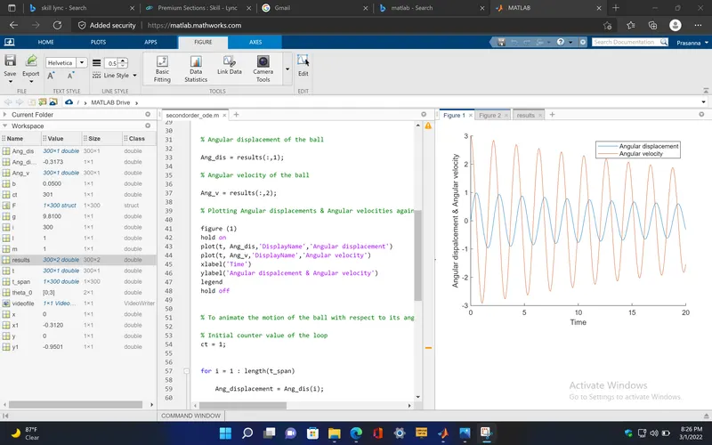
OUTPUT LINK :

YOUTUBE VIDEO LINK : https://youtu.be/do2cdqAIcwQ

EXPLANATION :

The Matlab uses the Fourth order Runge-Kutta method for solving the initial-value problems of first order ODEs. Since, the R-K method solves only for first order ODEs, for solving higher order ODEs(order greater than one), we have split the ODEs into No. of first order ODEs to solve it.

In this problem, for solving the second order ODE of a simple pendulum, first, we have to split it into two first order ODEs, one is displacement and the other is velocity.

The equation for the motion of a simple pendulum is derived from Newton's second law of motion, which is given as,

`d^2theta/dt^2 + b/m * d theta/dt + g/L * sin(theta) = 0`

Where,

b = damping co-efficient

m = mass of the ball (in 'kg')

g = acceleration due to gravity(in 'm/s^2')

L = length of the pendulum(in 'm')

theta = Angular displacement(in 'rad')

Rewriting the above equation into two first order ODEs,

If `theta = theta_1` and `d theta_1/dt = theta_2` , we get

`d theta/dt = theta_2`

`d^2 theta/dt^2 = d theta_2/dt`

Substuting the above values in equation, we get

`d theta_2/dt + b/m * theta_2 + g/L * sin(theta_1) = 0`

From the above equation, we get

`d theta_1/dt = theta_2`

`d theta_2/dt = -b/m * (theta_2) - g/L * sin(theta_1)`

In matrix form,

`[[d theta_1/dt],[d theta_2/dt]] = [[theta_2],[-b/m * theta_2 - g/L * sin(theta_1)]]`

PROGRAM EXPLANATION :

clear all - used to clear all the workspace variables.

close all - used to close all the previous figure windows if any.

clc - used to clear the command window.

m = 1; - Mass of the ball (in 'kg')

g = 9.81; - Acceleration due to gravity(in 'm/s^2')

l = 1; - Length of the pendulum(in 'm')

b = 0.05; - Damping co-efficient

theta_0 = [0 ; 3]; - at initial condition, when time = 0, Angular displacement = 0(in'm') & Angular velocity = 3(in 'rad/s')

t_span = linspace(0,20,300); - It is a row vector consisting 300 no. of evenly spaced values between 0 and 20.

[t, results] = ode45(@(t,theta) ode_func(t,theta,m,g,l,b),t_span,theta_0);

- 'ode45' is the in built matlab solver for ODEs, it takes three input arguments,

1. @(t,theta) ode_func(t,theta,m,g,l,b) - where the '@' indicates the function handle which has the inputs 't'(independent variable of the ODE) ant 'theta'(dependent variable of the ODE), 'ode_func(t,theta,m,g,l,b)' is seperate Matlab function code which takes in the values for the required variables and solves it using the function.

2. t_span indicates the integration limits for the ODE.

3. theta_0 indicates the initial condition(at t=0) of the angular displacement and angular velocity.

and the outputs were stored in, 't' which has the values for the time integration and 'results' which have the values of angular displacement and angular velocity for the given time range.

Ang_dis = results(:,1); - The first column in the 'results' have the values of the angular displacement.

Ang_v = results(:,2); - The second column in the 'results' have the values of the angular velocity.

Plotting Angular displacements & Angular velocities against time

figure (1)
hold on
plot(t, Ang_dis,'DisplayName','Angular displacement')
plot(t, Ang_v,'DisplayName','Angular velocity')
xlabel('Time')
ylabel('Angular dispalcement & Angular velocity')
legend
hold off

To animate the motion of the ball with respect to its angular displacement, 'for' loop is used.

ct = 1; - Initial counter value of the loop

for i = 1 : length(t_span)

Ang_displacement = Ang_dis(i); - for each value of 'i', the respective angular displacement value is stored in 'Ang_displacement' in the loop.

x = 0;
y = 0; - co-ordinate values for the fixed end of the pendulum.

x1 = l*sin(Ang_displacement);
y1 = -l*cos(Ang_displacement); - co-ordinate values for motion of the ball, which is calculated for each value of angular displacement in the loop.

figure(2) - for each value of 'i', 'figure 2' creates a plot using the 'plot' command below.

plot([x x1],[y y1],'linewidth',1.5,'Color','r','Marker','o','MarkerIndices',2,'markerfacecolor','m','markeredgecolor','k','MarkerSize',20)
axis([-1 1 -1.5 0])

F(ct) = getframe(gcf); - The plots in the 'figure 2' windows is captured as frames and stored in the value 'F'.

ct = ct + 1;

end

movie(F) - it creates the movie by the frames captured in 'F'.

videofile = VideoWriter('Simple_Pendulum.avi','Uncompressed AVI');
open(videofile)
writeVideo(videofile,F)
close(videofile)

ERRORS occurred while programming and its correction :

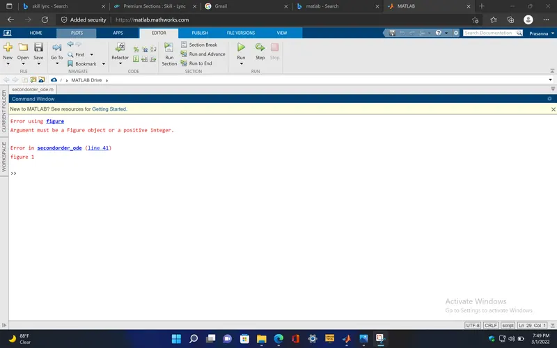
I have used 'figure 1' command in my script to create a figure window which gave me an error because the parenthesis was not included. So, I changed it to 'figure(1)'.