Week 3 - External flow simulation over an Ahmed body.
AIM :
To run a external flow simulation over an Ahmed body with the air flow velocity of 25 m/s using Ansys fluent.
OBJECTIVE :
- To create computational domain for the given Ahmed car body model in spaceclaim.
- To mesh the fluid domain with different mesh element size for different cases in order to do the grid independency test for those different cases.
- To run a external flow simulation over an Ahmed body by choosing the fluid as air and its properties, which flows at the inlet with velocity of 25 m/s.
- To find the drag co-efficient in the Ahmed body, and also to create velocity and pressure contours.
- To explain the reason for the negative pressure in the wake region.
- To explain the significance of the point of separation.
INTRODUCTION :
In this project, we are going to simulate the flow over an Ahmed body with the air velocity of 25 m/s to capture the wake region that is formed behind the Ahmed body, which causes the drag force to the Ahmed body due the pressure difference of air in that region.
Ahmed body and its importance:
It is a simplified car body which is created mainly for comparing and so validating the computationally simulated results with the experimental results in order to check whether the simulation results are correct, and so can perform the external flow analysis computationally to reduce the drag force on the car by capturing the wake region formed behind the car surface.
The Ahmed car body represents a generic car (passenger car) geometry which exhibits many of the flow features found in real-life cars despite its simplified geometry. The Ahmed body is a generic car model first proposed by Ahmed in 1984. All ground vehicles can be termed as bluff bodies moving close to the road surface. The analyzed body is able to capture the essential features of the flow which characterize modern cars.
CASE SETUP :
- In order to the choose the correct mesh element length, grid independency test is to be performed by choosing different mesh element size for running the simulation. The mesh element size which gives the accurate value for the co-efficient of drag and also takes less computational time is taken as the optimum mesh element size for this model.
- Here, to reduce the total number of mesh elements, create two computational domain for the Ahmed body, one domain closer to the Ahmed body which will have a finer mesh size to capture the wake region more accurately and enclosing it the other domain with coarse mesh in order to reduce the computational time.
- The fluid is taken as air with its properties which flows at the velocity of 25 m/s.
The following table shows the case setup with different mesh element size,
| CASE STUDY |
MESH ELEMENT SIZE (in ‘mm’) |
||
|
Larger domain |
Smaller domain |
Car bottom leg surface (circular) |
|
|
CASE - 1 |
250 |
100 |
5 |
|
CASE - 2 |
100 |
50 |
5 |
|
CASE - 3 (Split body) |
100 |
30 |
5 |
Since the Ahmed body is symmetric along its length, we can split the Ahmed body and perform simulation on half portion of the Ahmed body. This will reduce the number of mesh elements and so the computational time will also be reduced. Thus, giving the simulation results faster. In case 3, we use this approach since the total number of mesh elements will be higher because of the small mesh element size.
PROCEDURE :
CASE - 1 ( with mesh element size as 250mm and 100mm) :
PRE-PROCESSING :
- Import the given Ahmed body into spaceclaim from Ansys fluent and measure the dimensions of the given Ahmed body model.
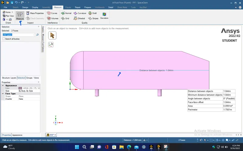
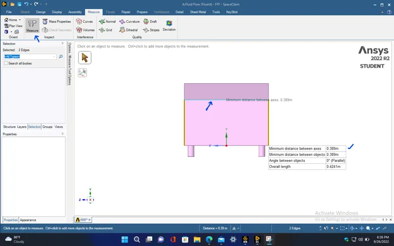
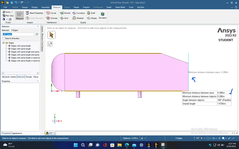
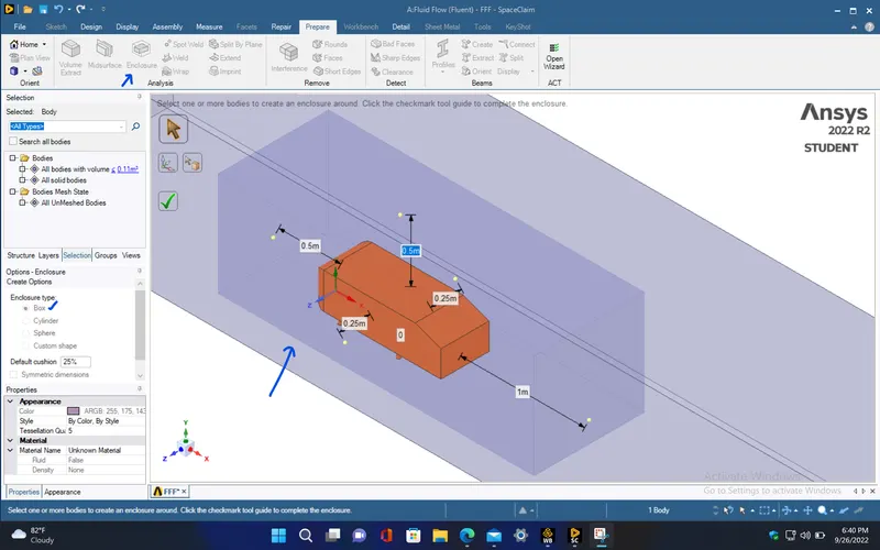
- Create the computational domain for the Ahmed body with respective distance from the Ahmed body as shown below,
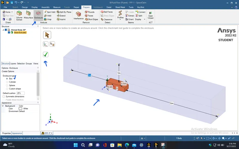
- Create another domain closer to the Ahmed body in order to get the accurate results near to the Ahmed body, which will have smaller mesh element length. This also reduces the computational time since we give larger mesh element length for the larger domain.
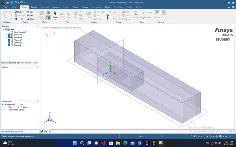
- Create planes to view the cross section of the domain.
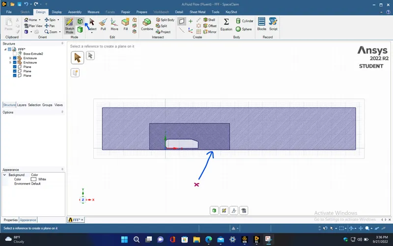
- From the below image, we can see that the larger domain volume is getting overlapped with smaller domain volume.
.
- In order to delete the overlapped region, use interference option which will auto detect the interfered region and delete it.
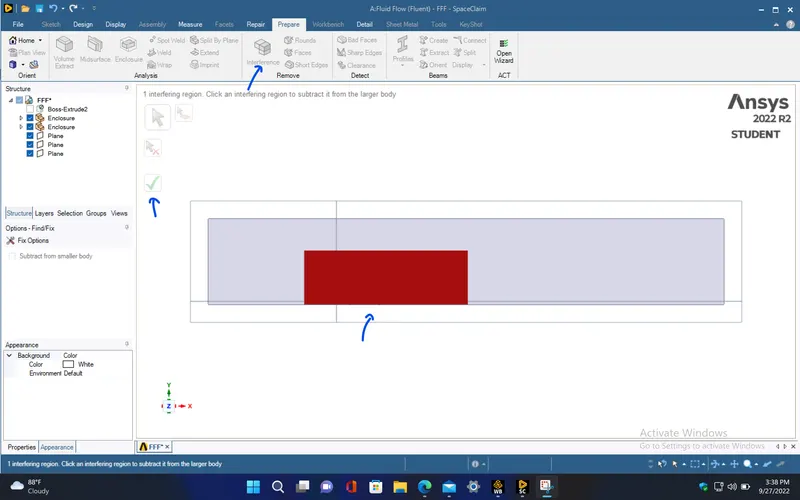
- Now, the cross sectional view is not showing any overlapped regions.
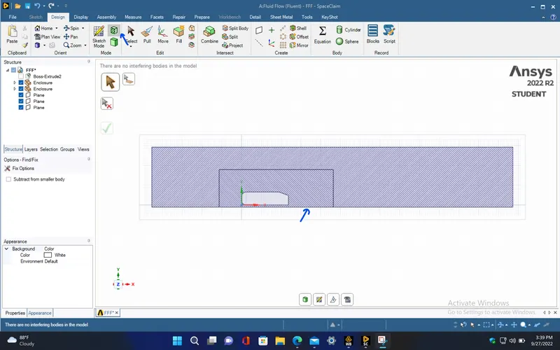
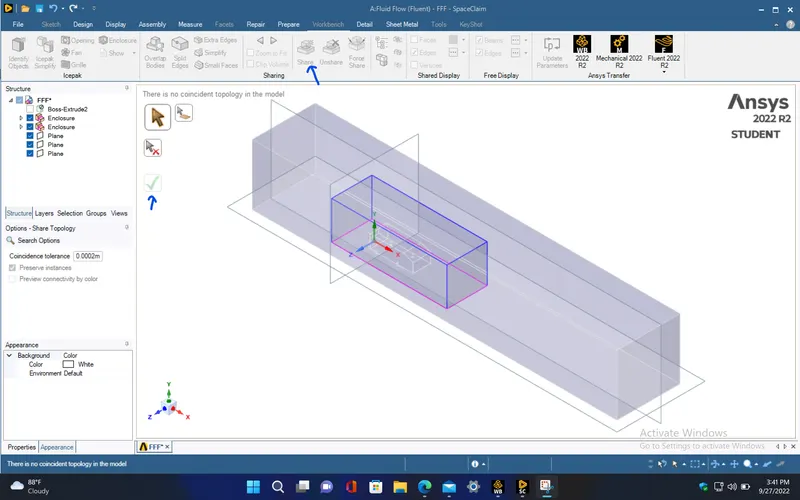
- Since the smaller domain is enclosed with larger domain, the topology is shared between the two domains. This shares common node points between the domains while meshing.
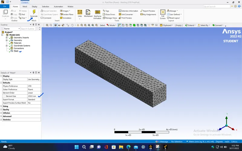
- Now, close the spaceclaim and open the mesh window from Ansys fluent, give the mesh element size as 250 mm and generate mesh.
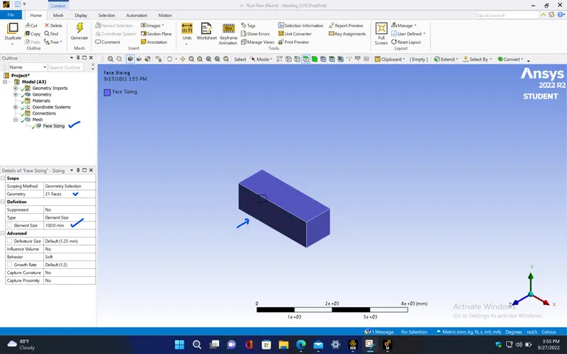
- Insert the sizing for the smaller domain with mesh element size as 100 mm.
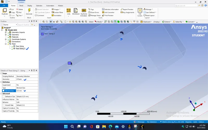
- Now, again insert sizing for the bottom circular surfaces with mesh element size as 5 mm in order to capture the circular surface properly.
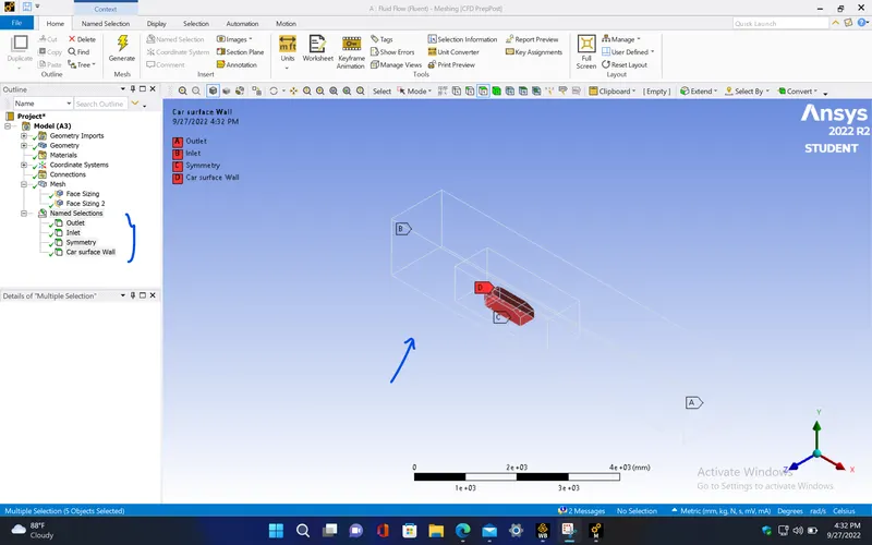
- Give required names for the every regions.
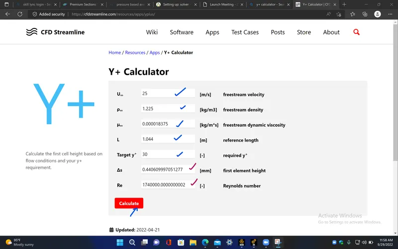
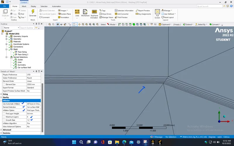
- Here, Y+ value is taken as 30 to calculate the first layer thickness of the inflation layer. Thus, from the Y+ calculator, we get the first layer thickness as 0.4 mm
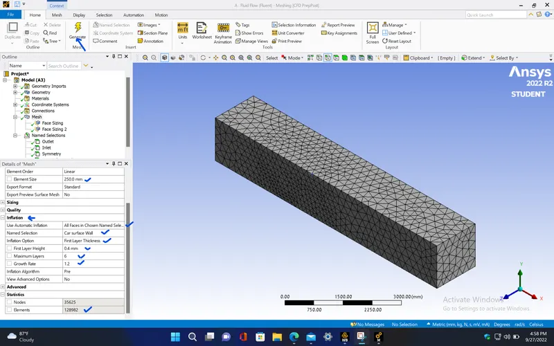
- Inflation layer also called as boundary layer, is created in order to capture the Ahmed body geometry accurately by generating the structured mesh over the Ahmed body. Choose inflation at the car wall surface and give the first layer thickness as 0.4 mm and maximum number of layers as 6.
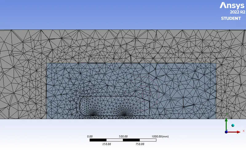
|
Cells |
Faces |
Nodes |
|
128982 |
280359 |
35625 |
SETUP AND SOLVING :
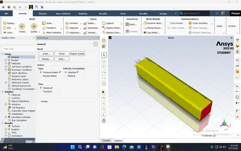
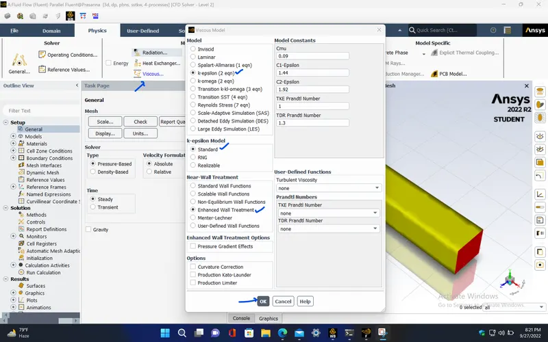
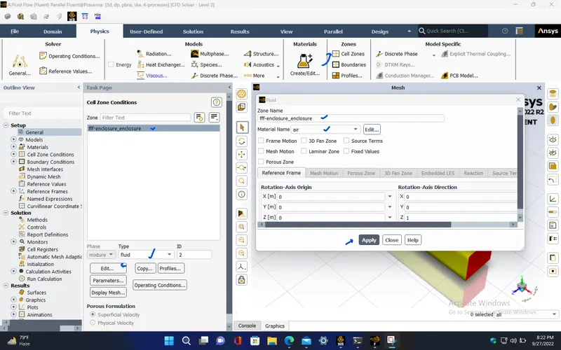
- Open setup window and give the following parameters.
|
Model |
Settings |
|
Space |
3D |
|
Model |
Settings |
|
Time |
Steady |
|
Viscous |
Standard k-epsilon turbulence model |
|
Wall Treatment |
Enhanced Wall Treatment |
MATERIAL PROPERTIES :
|
Fluid |
air |
|
Density |
1.225 kg/m^3 |
|
Cp (Specific Heat) |
1006.43 J/(kg K) |
|
Thermal Conductivity |
0.0242 W/(m K) |
|
Viscosity |
1.7894e-05 kg/(m s) |
|
Molecular Weight |
28.966 kg/kmol |
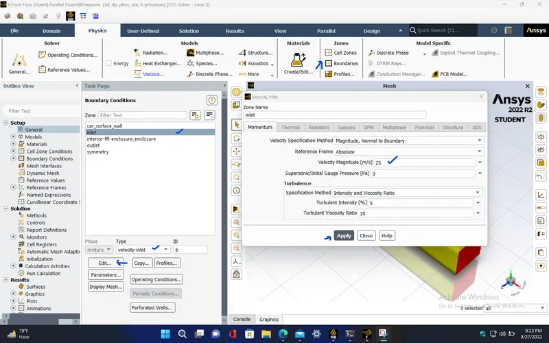
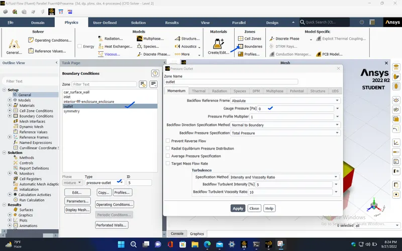
BOUNDARY CONDITIONS :
|
inlet |
|
|
Velocity Specification Method |
Magnitude, Normal to Boundary |
|
Reference Frame |
Absolute |
|
Velocity Magnitude [m/s] |
25 |
|
outlet |
|
|
Backflow Reference Frame |
Absolute |
|
Gauge Pressure [Pa] |
0 |
|
Backflow Direction Specification Method |
Normal to Boundary |
|
Symmetry |
|
|
symmetry |
symmetry |
|
car_surface_wall |
|
|
Wall Motion |
Stationary Wall |
|
Shear Boundary Condition |
No Slip |
REFERENCE VALUES :
|
Area |
0.131482 m^2 |
|
Density |
1.225 kg/m^3 |
|
Enthalpy |
0 J/kg |
|
Length |
1.044 m |
|
Pressure |
0 Pa |
|
Temperature |
288.16 K |
|
Velocity |
25 m/s |
|
Viscosity |
1.7894e-05 kg/(m s) |
|
Ratio of Specific Heats |
1.4 |
|
Yplus for Heat Tran. Coef. |
300 |
|
Reference Zone |
fff-enclosure_enclosure |
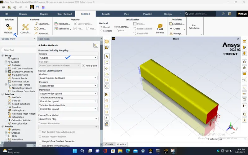
SOLVER :
|
Pressure-Velocity Coupling |
|
|
Type |
Coupled |
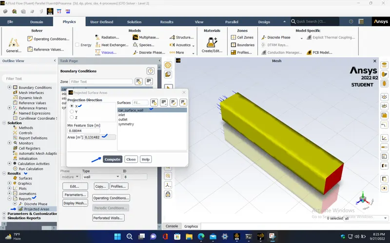
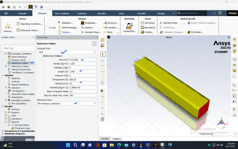
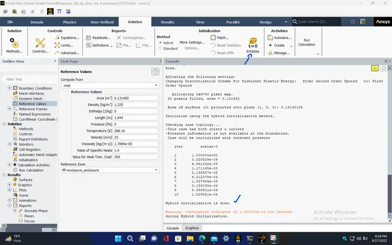
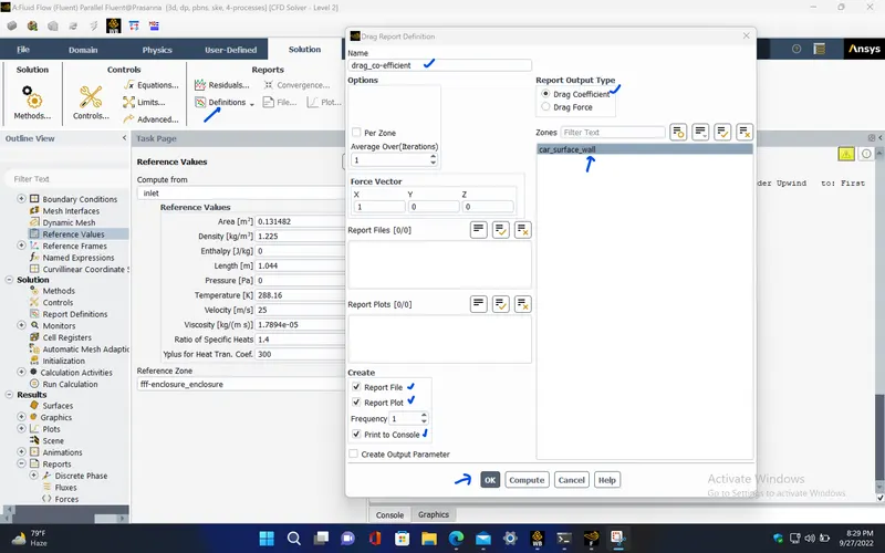
RESIDUAL PLOT :
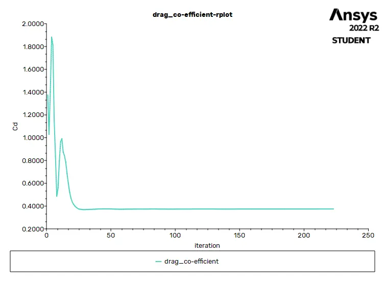
DRAG CO-EFFICIENT PLOT :
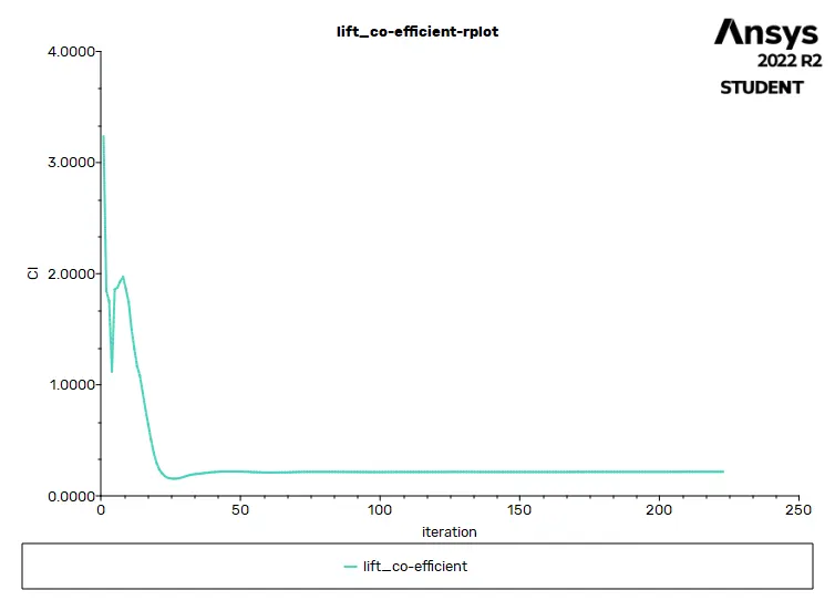
LIFT CO-EFFICIENT PLOT :
SOLUTION STATUS :
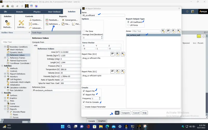
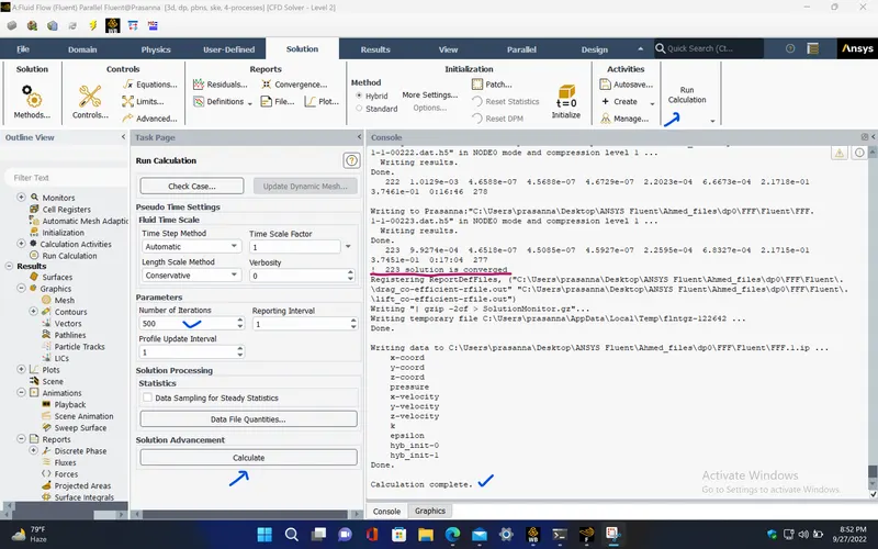
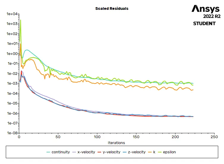
- From the above plots, we see that the solution got converged at 223th iteration since the rate at which residuals, velocity, drag co-efficient and lift co-efficient changes becomes constant over iteration.
Number of iteration - 223
|
Value |
Absolute Criteria |
Convergence Status |
|
|
continuity |
0.0009927442 |
0.001 |
Converged |
|
x-velocity |
4.651831e-07 |
0.001 |
Converged |
|
y-velocity |
4.508489e-07 |
0.001 |
Converged |
|
z-velocity |
4.592696e-07 |
0.001 |
Converged |
|
k |
0.0002259476 |
0.001 |
Converged |
|
epsilon |
0.000683269 |
0.001 |
Converged |
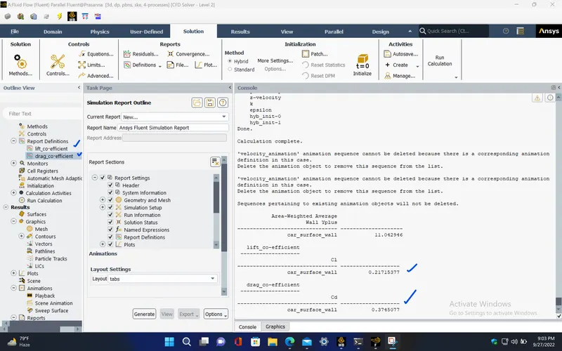
REPORT DEFINITIONS :
|
lift_co-efficient |
0.2171538 |
|
drag_co-efficient |
0.3745077 |
POST PROCESSING :
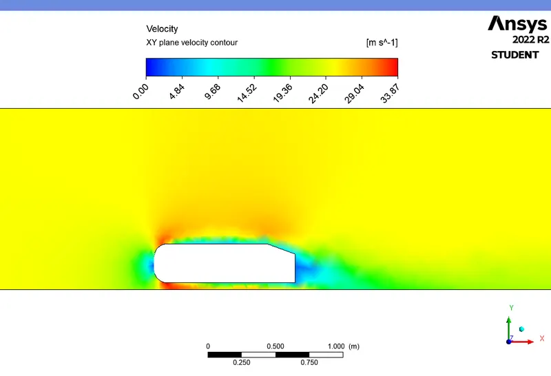
VELOCITY CONTOUR :
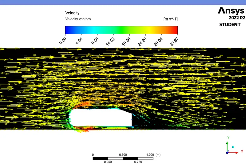
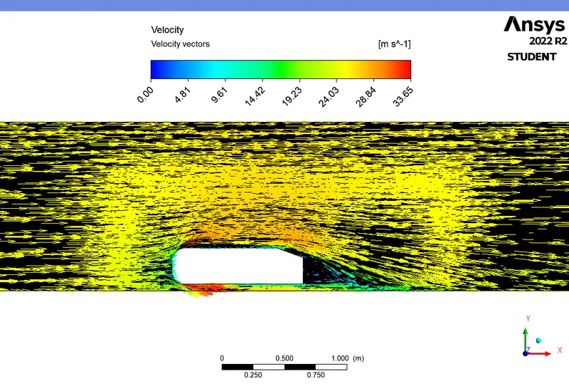
VELOCITY VECTOR :
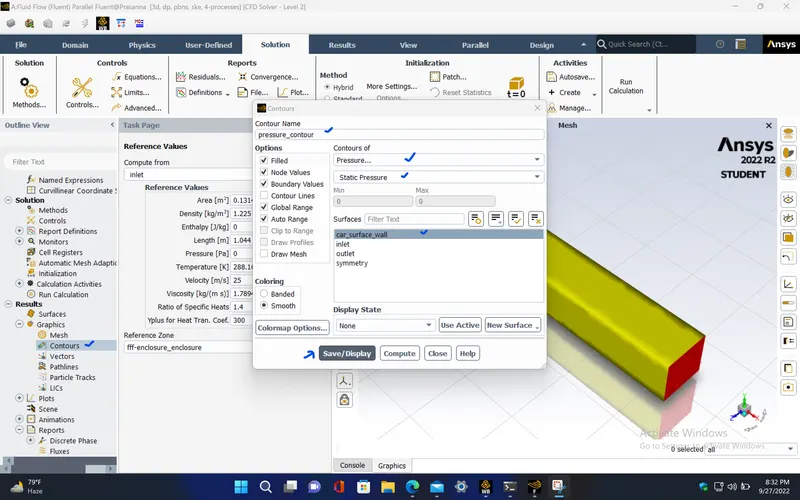
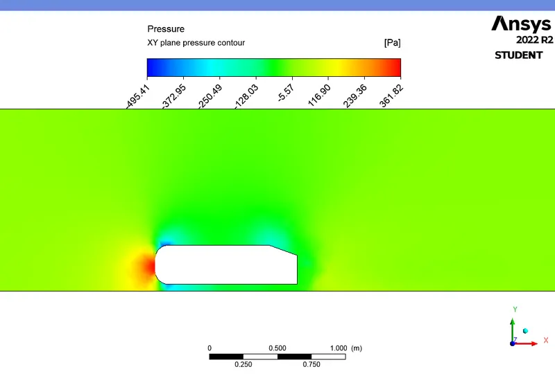
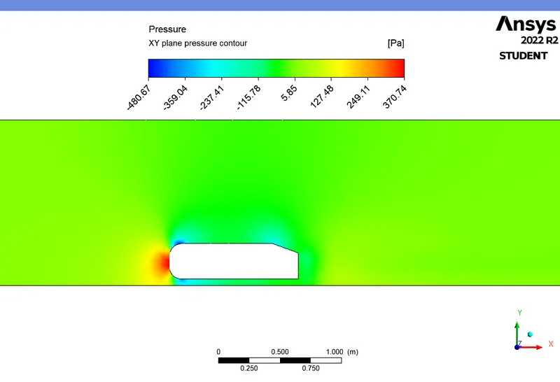
PRESSURE CONTOUR :
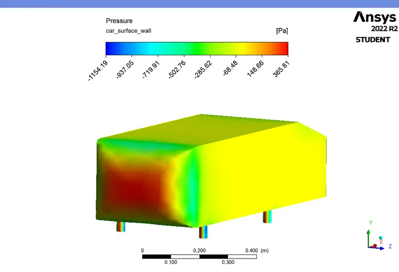
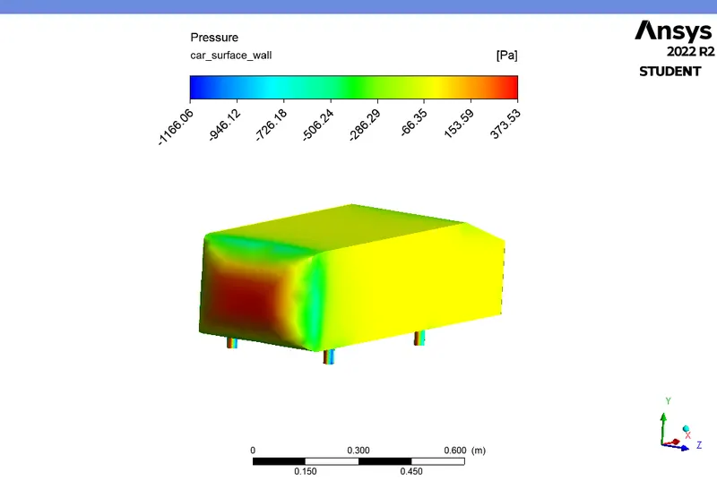
PRESSURE CONTOUR AT AHMED BODY :
CASE - 2 ( with mesh element size as 100mm and 50mm) :
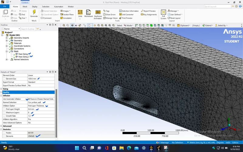
- Repeat the same procedure as done before, but now with changing the mesh element size.
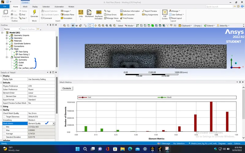
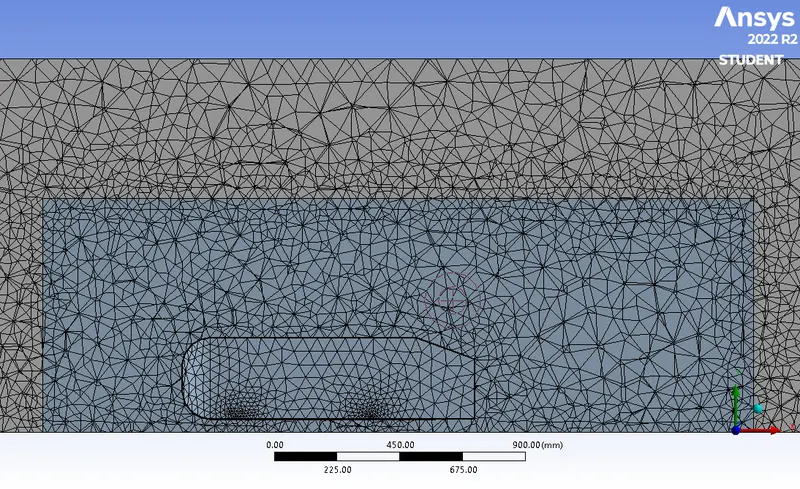
|
Cells |
Faces |
Nodes |
|
294549 |
616860 |
66159 |
SETUP AND SOLVING :
- Open setup window and give the following parameters.
|
Model |
Settings |
|
Space |
3D |
|
Model |
Settings |
|
Time |
Steady |
|
Viscous |
Standard k-epsilon turbulence model |
|
Wall Treatment |
Enhanced Wall Treatment |
MATERIAL PROPERTIES :
|
Fluid |
air |
|
Density |
1.225 kg/m^3 |
|
Cp (Specific Heat) |
1006.43 J/(kg K) |
|
Thermal Conductivity |
0.0242 W/(m K) |
|
Viscosity |
1.7894e-05 kg/(m s) |
|
Molecular Weight |
28.966 kg/kmol |
BOUNDARY CONDITIONS :
|
inlet |
|
|
Velocity Specification Method |
Magnitude, Normal to Boundary |
|
Reference Frame |
Absolute |
|
Velocity Magnitude [m/s] |
25 |
|
Supersonic/Initial Gauge Pressure [Pa] |
0 |
|
outlet |
|
|
Backflow Reference Frame |
Absolute |
|
Gauge Pressure [Pa] |
0 |
|
Symmetry |
|
|
symmetry |
symmetry |
|
car_surface_wall |
|
|
Wall Motion |
Stationary Wall |
|
Shear Boundary Condition |
No Slip |
REFERENCE VALUES :
|
Area |
0.131482 m^2 |
|
Density |
1.225 kg/m^3 |
|
Enthalpy |
0 J/kg |
|
Length |
1.044 m |
|
Pressure |
0 Pa |
|
Temperature |
288.16 K |
|
Velocity |
25 m/s |
|
Viscosity |
1.7894e-05 kg/(m s) |
|
Ratio of Specific Heats |
1.4 |
|
Yplus for Heat Tran. Coef. |
300 |
|
Reference Zone |
fff-enclosure_enclosure |
SOLVER :
|
Pressure-Velocity Coupling |
|
|
Type |
Coupled |
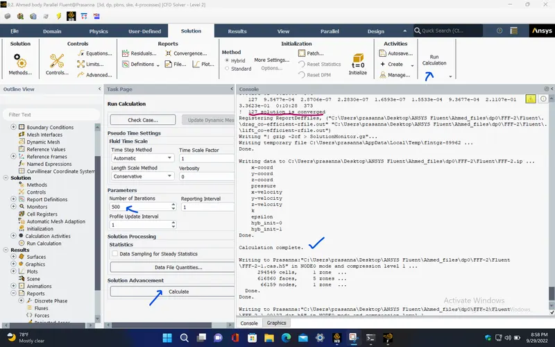
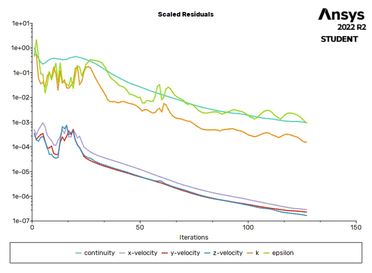
RESIDUAL PLOT :
DRAG CO-EFFICIENT PLOT :
LIFT CO-EFFICIENT PLOT :
SOLUTION STATUS :
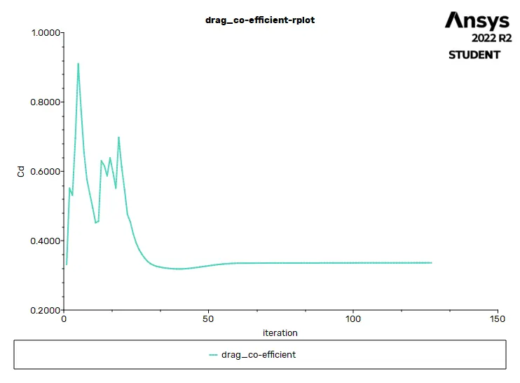
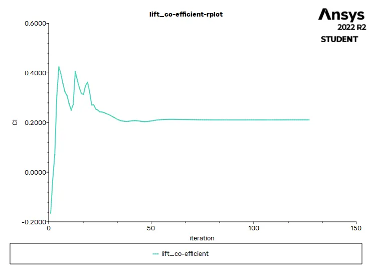
- From the above plots, we see that the solution got converged at 127th iteration since the rate at which residuals, velocity, drag co-efficient and lift co-efficient changes becomes constant over iteration.
Number of iteration - 127
|
Value |
Absolute Criteria |
Convergence Status |
|
|
continuity |
0.0009547684 |
0.001 |
Converged |
|
x-velocity |
2.870603e-07 |
0.001 |
Converged |
|
y-velocity |
2.282991e-07 |
0.001 |
Converged |
|
z-velocity |
1.659263e-07 |
0.001 |
Converged |
|
k |
0.0001553275 |
0.001 |
Converged |
|
epsilon |
0.0009367693 |
0.001 |
Converged |
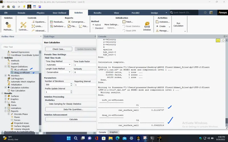
REPORT DEFINITIONS :
|
lift_co-efficient |
0.2110674 |
|
drag_co-efficient |
0.3362251 |
POST PROCESSING :
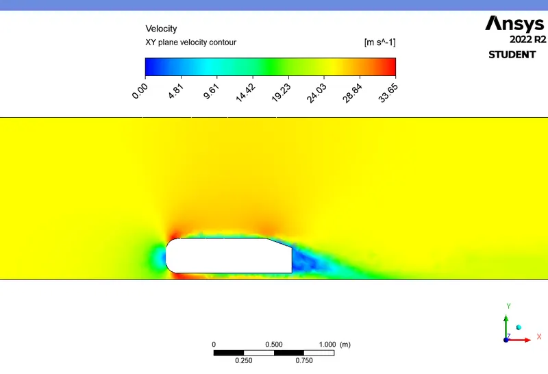
VELOCITY CONTOUR :
VELOCITY VECTOR :
PRESSURE CONTOUR :
PRESSURE CONTOUR AT AHMED BODY :
CASE - 3 (Split body, with mesh element size as 100mm and 30mm) :
PRE-PROCESSING :
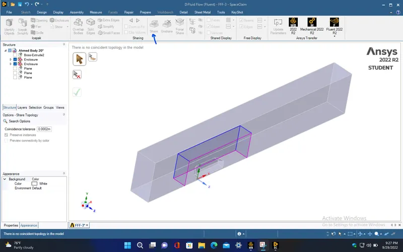
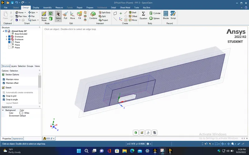
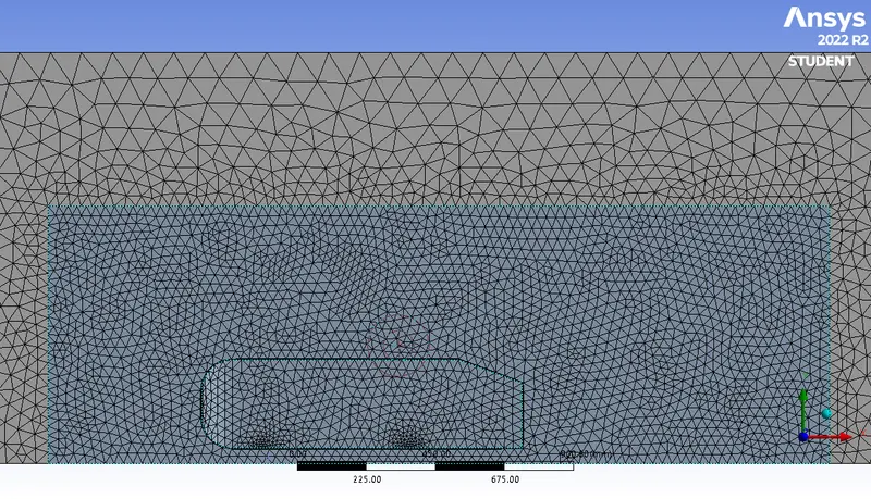
- After creating computational domains in spaceclaim, create planes.use split body option under workbench, select the entire body and then, select the cutting plane as XY plane. Now, delete the half portion of the body.
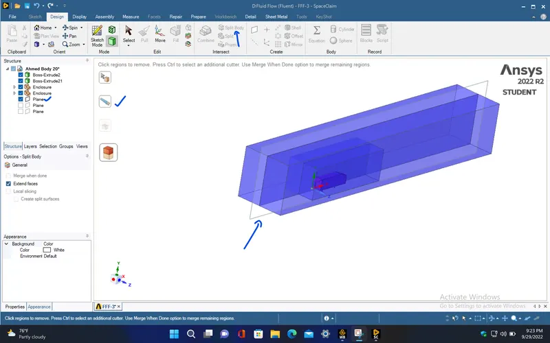
- Perform the share topology.
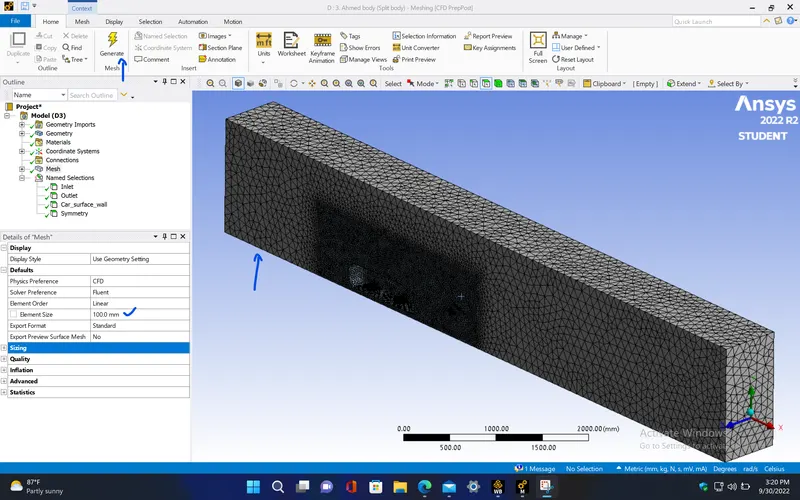
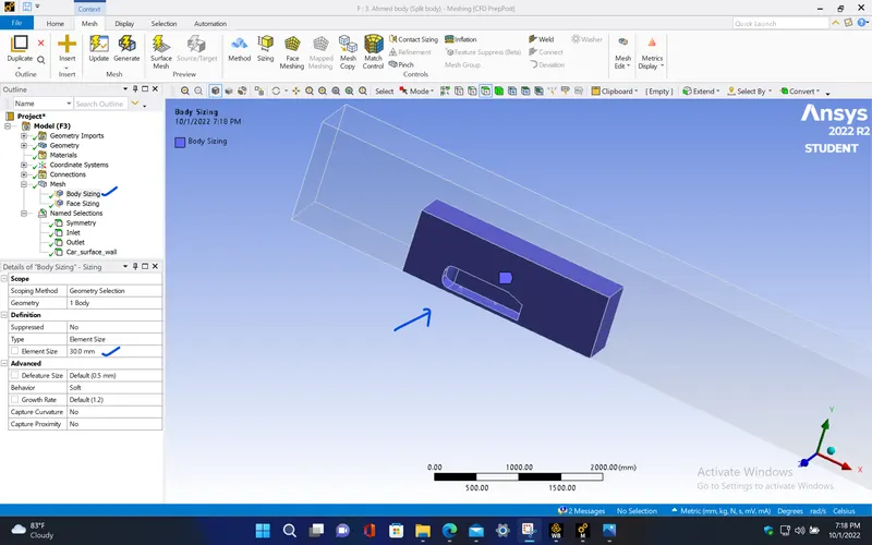
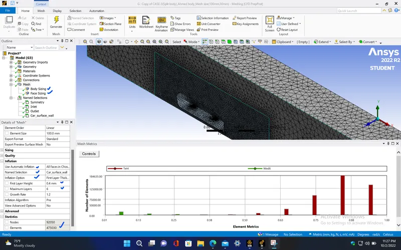
- Now, open mesh window and select the required mesh element size as described.
|
Cells |
Faces |
Nodes |
|
475030 |
971132 |
92050 |
SETUP AND SOLVING :
- Open setup window and give the following parameters.
|
Model |
Settings |
|
Space |
3D |
|
Model |
Settings |
|
Time |
Steady |
|
Viscous |
Standard k-epsilon turbulence model |
|
Wall Treatment |
Enhanced Wall Treatment |
MATERIAL PROPERTIES :
|
Fluid |
air |
|
Density |
1.225 kg/m^3 |
|
Cp (Specific Heat) |
1006.43 J/(kg K) |
|
Thermal Conductivity |
0.0242 W/(m K) |
|
Viscosity |
1.7894e-05 kg/(m s) |
|
Molecular Weight |
28.966 kg/kmol |
|
Cp (Specific Heat) |
871 J/(kg K) |
BOUNDARY CONDITIONS :
|
inlet |
|
|
Velocity Specification Method |
Magnitude, Normal to Boundary |
|
Reference Frame |
Absolute |
|
Velocity Magnitude [m/s] |
25 |
|
outlet |
|
|
Backflow Reference Frame |
Absolute |
|
Gauge Pressure [Pa] |
0 |
|
Backflow Direction Specification Method |
Normal to Boundary |
|
Symmetry |
|
|
symmetry |
symmetry |
|
car_surface_wall |
|
|
Wall Motion |
Stationary Wall |
|
Shear Boundary Condition |
No Slip |
REFERENCE VALUES :
|
Area |
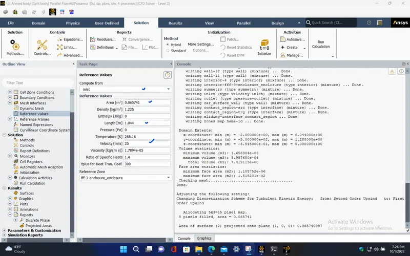
0.065741 m^2 |
|
Density |
1.225 kg/m^3 |
|
Enthalpy |
0 J/kg |
|
Length |
1.044 m |
|
Pressure |
0 Pa |
|
Temperature |
288.16 K |
|
Velocity |
25 m/s |
|
Viscosity |
1.7894e-05 kg/(m s) |
|
Ratio of Specific Heats |
1.4 |
|
Yplus for Heat Tran. Coef. |
300 |
|
Reference Zone |
fff-3-enclosure_enclosure |
SOLVER :
|
Pressure-Velocity Coupling |
|
|
Type |
Coupled |
RESIDUAL PLOT :
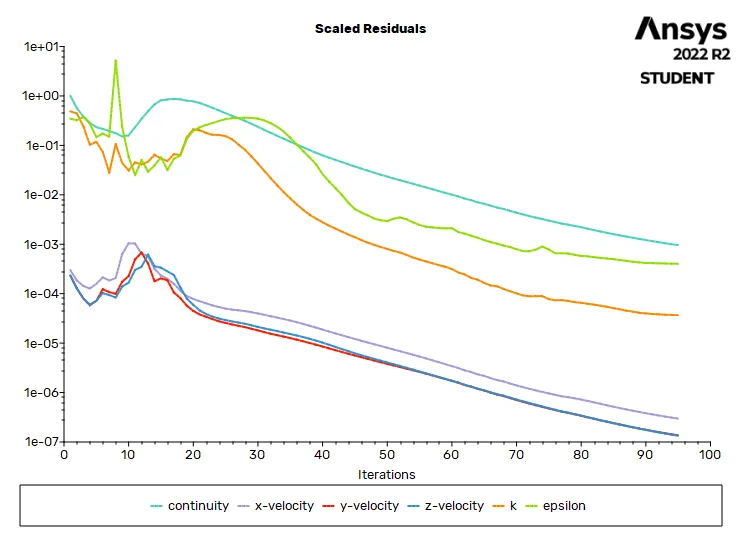
DRAG CO-EFFICIENT PLOT :
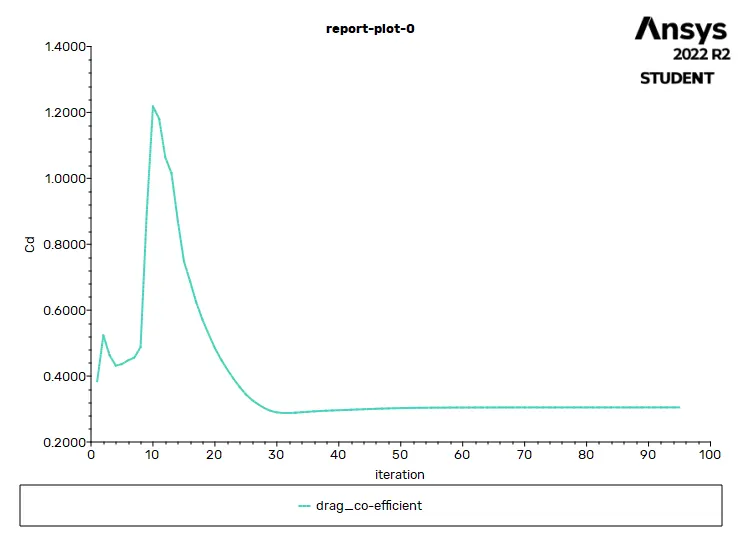
LIFT CO-EFFICIENT :
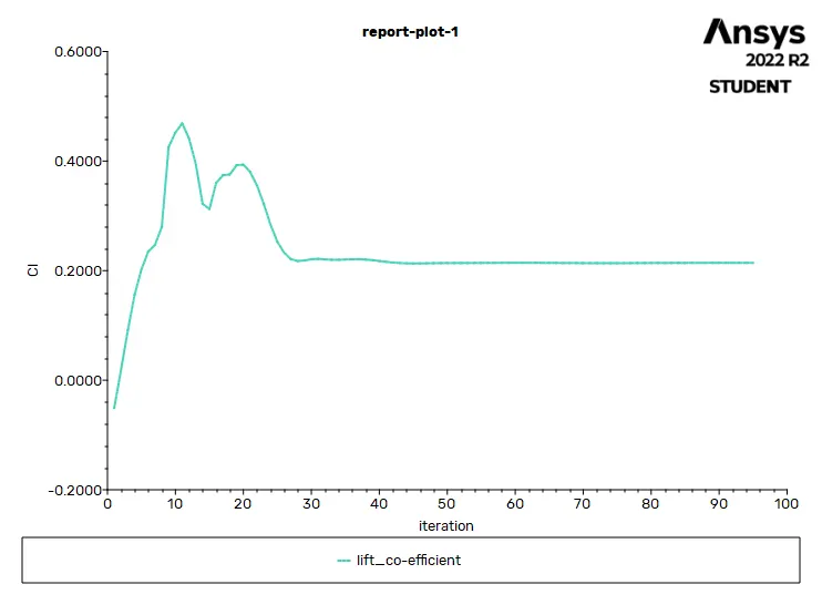
SOLUTION STATUS :
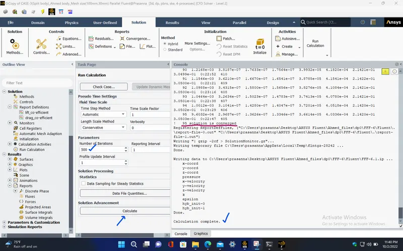
- From the above plots, we see that the solution got converged at 99 th iteration since the rate at which residuals, velocity, drag co-efficient and lift co-efficient changes becomes constant over iteration.
Number of iteration - 99
|
Value |
Absolute Criteria |
Convergence Status |
|
|
continuity |
0.0009603193 |
0.001 |
Converged |
|
x-velocity |
2.968656e-07 |
0.001 |
Converged |
|
y-velocity |
1.36265e-07 |
0.001 |
Converged |
|
z-velocity |
1.334642e-07 |
0.001 |
Converged |
|
k |
3.661356e-05 |
0.001 |
Converged |
|
epsilon |
0.0004033633 |
0.001 |
Converged |
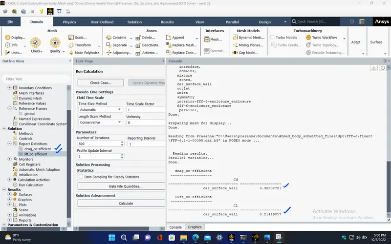
REPORT DEFINITIONS :
|
drag_co-efficient |
0.3050272 |
|
lift_co-efficient |
0.2141986 |
POST PROCESSING :
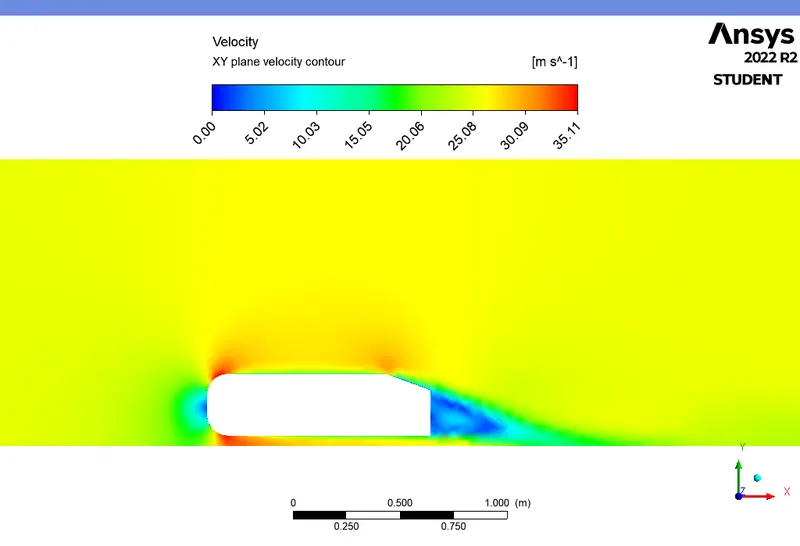
VELOCITY CONTOUR :
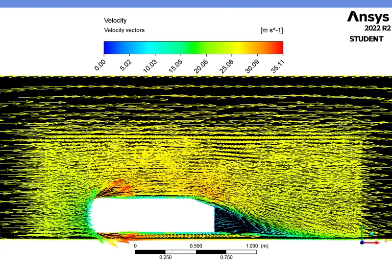
VELOCITY VECTOR :
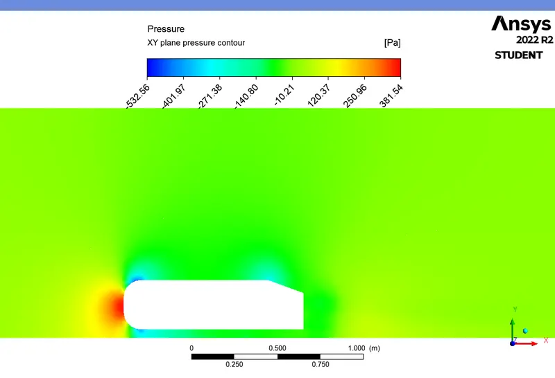
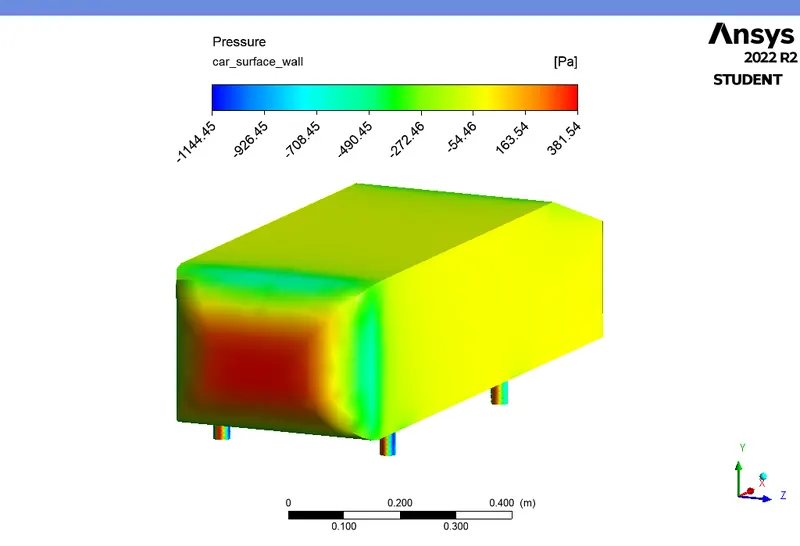
PRESSURE CONTOUR :
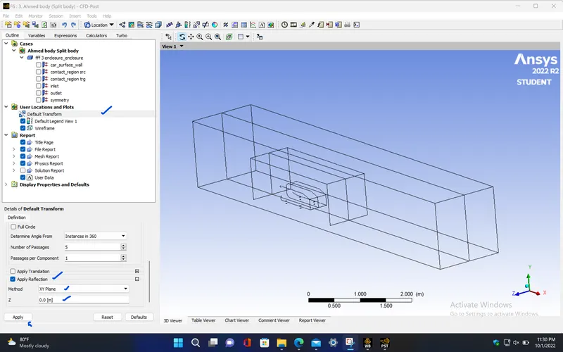
- To transform the half portion into a whole body, use reflection under transform option.
PRESSURE CONTOUR AT AHMED BODY :
RESULT :
Google drive link for the file :
https://drive.google.com/file/d/1ptyNicY3Q0EF94_UZstRVdx_P_VysIRX/view?usp=sharing
VELOCITY CHART :
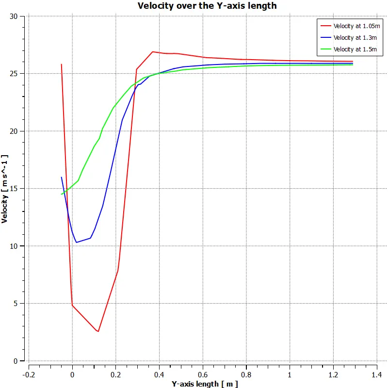
CASE - 1 ( with mesh element size as 250mm and 100mm) :
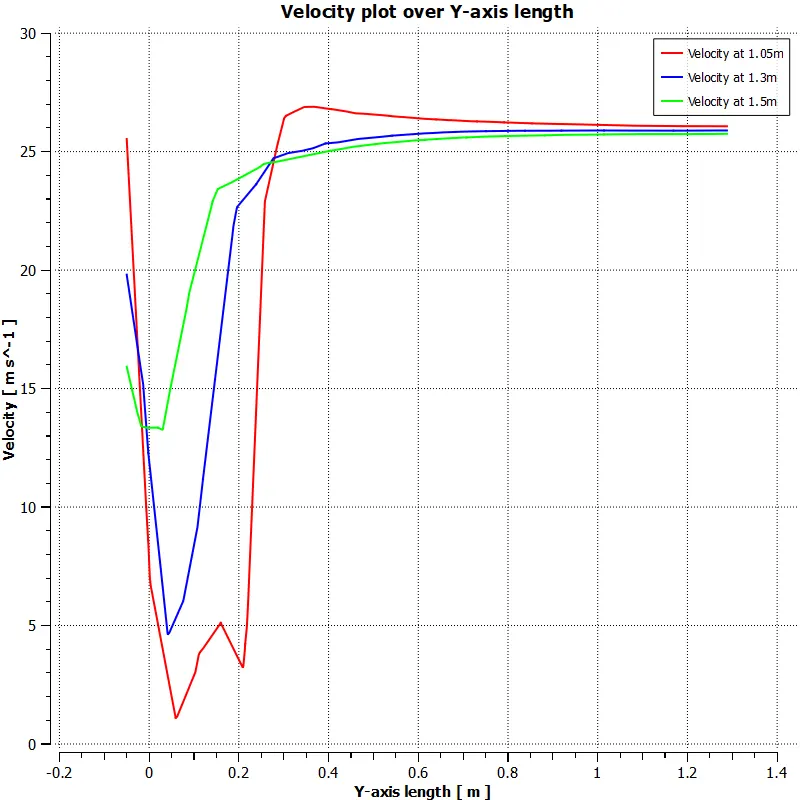
CASE - 2 ( with mesh element size as 100mm and 50mm) :
CASE - 3 (Split body, with mesh element size as 100mm and 30mm) :
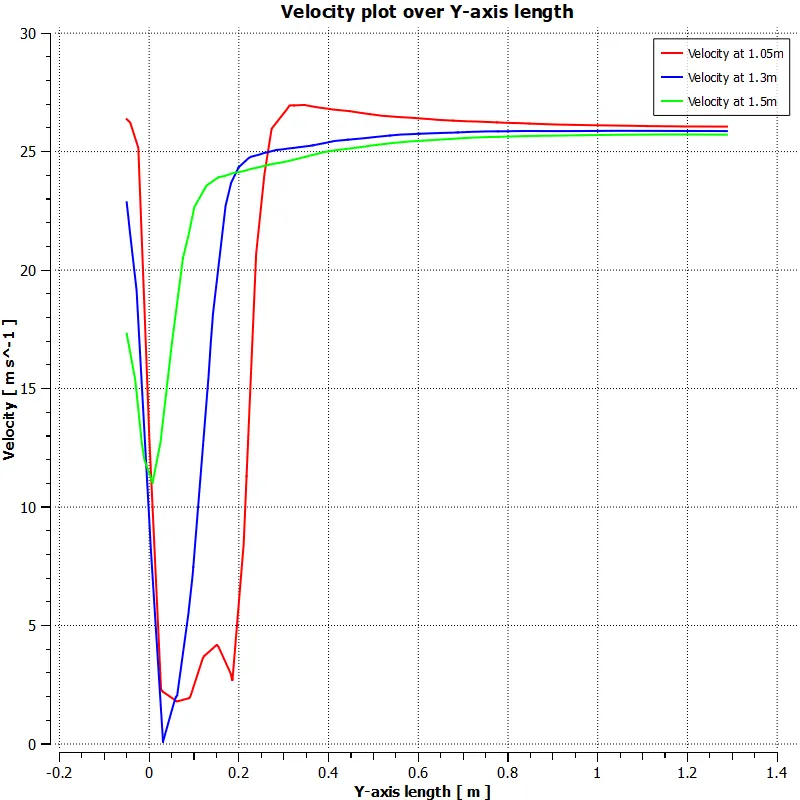
- From the above plots, we can see that for all the cases,If we consider the velocity over the vertical axis (y-axis) length behind the Ahmed body as the y-axis length increases, the velocity also increases from almost 0 (at wake region) to the 25 m/s (freestream velocity) and also if we consider verlocity over the y-axis length at different distance from x-axis, we can observe that, as we increase the distance from x-axis, the change in velocity over y-axis length decreases and tends almost towards a constant value.
CONCLUSION :
Grid independency test :
|
MESH ELEMENT SIZE ( in ‘mm’ ) |
NUMBER OF MESH ELEMENTS |
COEFFICIENT OF DRAG |
COEFFICIENT OF LIFT |
||
|
Larger domain |
Smaller domain |
||||
|
CASE - 1 |
250 |
100 |
128982 |
0.3745077 |
0.2171538 |
|
CASE - 2 |
100 |
50 |
294549 |
0.3362251 |
0.2110674 |
| CASE - 3 | 100 | 30 | 475030 | 0.3050272 | 0.2141986 |
- From the above table, we can see that the case 2 gives the optimum result for co-efficient of drag(Cd) and lift (Cl) as 0.336 and 0.211 respectively with fewer number of mesh elements and so will take lesser computational time compared to other cases.
Velocity vector :
Reason for the negative pressure in the wake region :
Wake region is the region where velocity gets decreased due to the sudden blunt geometry change behind the Ahmed body. The air flow nearer to the surface will undergo higher resistive force with higher velocity gradient compared to air flowing far away from the surface. Thus, the air flowing away from the surface tend to keep the air flowing with higher velocity. This is due to the viscosity of the fluid (air). Thus there is pressure difference occurs behind the Ahmed body due to which the pressure flows from the high pressure region to low pressure region.
Significance of the point of separation :
Point of seperation occurs behind the Ahmed car body due to higher pressure gradient. This causes the resistive force called the drag force on the Ahmed body as pressure flows from high pressure region to low pressure region. The air flow nearer to the surface will have almost zero velocity with higher velocity gradient whereas the flow away from the surface will have a higher velocity. This will causes the flow seperation behind the Ahmed body due the blunt geometry.